0. Code to run to set up your computer.
# Update Packages
# update.packages(ask = FALSE, repos='https://cran.csiro.au/', dependencies = TRUE)

# Install Packages
if(!require(dplyr)) {install.packages("sjlabelled", repos='https://cran.csiro.au/', dependencies=TRUE)}
if(!require(sjlabelled)) {install.packages("sjlabelled", repos='https://cran.csiro.au/', dependencies=TRUE)}
if(!require(sjmisc)) {install.packages("sjmisc", repos='https://cran.csiro.au/', dependencies=TRUE)}
if(!require(sjstats)) {install.packages("sjstats", repos='https://cran.csiro.au/', dependencies=TRUE)}
if(!require(sjPlot)) {install.packages("sjlabelled", repos='https://cran.csiro.au/', dependencies=TRUE)}
if(!require(summarytools)) {install.packages("summarytools", repos='https://cran.csiro.au/', dependencies=TRUE)}
if(!require(ggplot2)) {install.packages("ggplot2", repos='https://cran.csiro.au/', dependencies= TRUE)}
if(!require(ggthemes)) {install.packages("ggthemes", repos='https://cran.csiro.au/', dependencies= TRUE)}
if (!require(GPArotation)) install.packages("GPArotation", repos='https://cran.csiro.au/', dependencies = TRUE)
if (!require(psych)) install.packages("psych", repos='https://cran.csiro.au/', dependencies = TRUE)
if (!require(ggrepel)) install.packages("ggrepel", repos='https://cran.csiro.au/', dependencies = TRUE)


# Load packages into memory
library(dplyr)
library(sjlabelled)
library(sjmisc)
library(sjstats)
library(sjPlot)
library(summarytools)
library(ggplot2)
library(ggthemes)
library(GPArotation)
library(psych)
library(ggrepel)

# Turn off scientific notation
options(digits=5, scipen=15)

# Stop View from overloading memory with a large datasets
RStudioView <- View
View <- function(x) {
  if ("data.frame" %in% class(x)) { RStudioView(x[1:500,]) } else { RStudioView(x) }
}

# Datasets
# Example 1: Crime Dataset
lga <- readRDS(url("https://mqsociology.github.io/learn-r/soci832/nsw-lga-crime.RDS"))
# extract just the crimes from crime dataset
first <- which( colnames(lga)=="astdomviol" )
last <- which(colnames(lga)=="transport")
crimes <- lga[, first:last ]

# Example 2: AuSSA Dataset
aus2012 <- readRDS(url("https://mqsociology.github.io/learn-r/soci832/aussa2012.RDS"))

# Example 3: Australian Electoral Survey
aes_full  <- sjlabelled::read_spss(url("https://methods101.com/data/2013_aes_full.sav"))
# Codebook
browseURL("https://mqsociology.github.io/learn-r/soci832/aes_full_codebook.html")
Analyse to find out how many factors to choose
psych::fa.parallel(attitudes, fm="pa", fa="fa", use="pairwise")
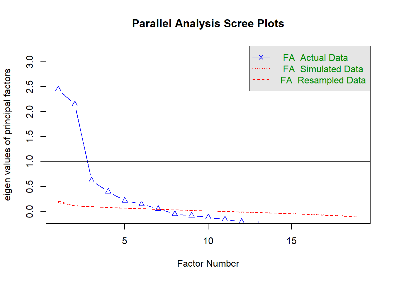
## Parallel analysis suggests that the number of factors = 7 and the number of components = NA
Seven Factor Solution: Oblique (promax rotation)
Run analysis
results.1 <- fa(r = attitudes, nfactors = 7, rotate = "promax", fm="pa")
## maximum iteration exceeded
## Warning in fac(r = r, nfactors = nfactors, n.obs = n.obs, rotate =
## rotate, : A loading greater than abs(1) was detected. Examine the loadings
## carefully.
results.1
## Factor Analysis using method =  pa
## Call: fa(r = attitudes, nfactors = 7, rotate = "promax", fm = "pa")
##
##  Warning: A Heywood case was detected.
## Standardized loadings (pattern matrix) based upon correlation matrix
##            PA2   PA6   PA4   PA3   PA7   PA1   PA5   h2   u2 com
## d1tax     0.02 -0.08 -0.06  0.07  0.60  0.02 -0.03 0.32 0.68 1.1
## d1immig   0.07 -0.07  0.67  0.02  0.07  0.09 -0.01 0.53 0.47 1.1
## d1educ   -0.06 -0.02  0.05  0.00  0.07  0.72 -0.01 0.56 0.44 1.0
## d1envir   0.02  0.59 -0.03 -0.03 -0.07  0.32 -0.03 0.58 0.42 1.6
## d1indrel -0.05  0.08  0.00  0.04  0.47  0.13  0.01 0.30 0.70 1.3
## d1health  0.07  0.01  0.02  0.01  0.17  0.55  0.01 0.42 0.58 1.2
## d1reas   -0.07  0.01  0.97 -0.01 -0.18  0.02  0.00 0.80 0.20 1.1
## d1global  0.11  1.02 -0.08 -0.05 -0.14  0.01  0.00 0.86 0.14 1.1
## d1carbon -0.04  0.42  0.11  0.01  0.29 -0.17  0.03 0.30 0.70 2.4
## d1econo  -0.02 -0.04 -0.03 -0.05  0.54  0.08  0.03 0.31 0.69 1.1
## e6deathp  0.80  0.03 -0.04  0.17 -0.04 -0.01 -0.02 0.54 0.46 1.1
## e6marij  -0.06  0.06  0.00  0.07 -0.02 -0.05 -0.26 0.11 0.89 1.5
## e6lawbrk  0.72  0.06 -0.03  0.04 -0.08  0.09  0.01 0.44 0.56 1.1
## e6pref    0.14 -0.10  0.00  0.99  0.13 -0.14  0.00 0.80 0.20 1.1
## e6boats   0.64 -0.07  0.07  0.13  0.06 -0.13  0.12 0.57 0.43 1.3
## e6same    0.06  0.08 -0.01  0.06 -0.02 -0.07  0.91 0.81 0.19 1.0
## e6white  -0.21  0.02 -0.01  0.20 -0.06  0.04  0.13 0.12 0.88 3.0
## e6ethnic  0.33  0.04  0.00 -0.09  0.01  0.01  0.08 0.16 0.84 1.3
## e6opp     0.08  0.03  0.01  0.47 -0.03  0.12 -0.09 0.29 0.71 1.3
##
##                        PA2  PA6  PA4  PA3  PA7  PA1  PA5
## SS loadings           1.69 1.52 1.35 1.11 1.02 1.16 0.98
## Proportion Var        0.09 0.08 0.07 0.06 0.05 0.06 0.05
## Cumulative Var        0.09 0.17 0.24 0.30 0.35 0.41 0.46
## Proportion Explained  0.19 0.17 0.15 0.13 0.12 0.13 0.11
## Cumulative Proportion 0.19 0.36 0.52 0.64 0.76 0.89 1.00
##
##  With factor correlations of
##       PA2   PA6   PA4   PA3   PA7   PA1   PA5
## PA2  1.00 -0.35  0.22 -0.26  0.46 -0.05  0.39
## PA6 -0.35  1.00  0.29  0.38  0.19  0.47 -0.33
## PA4  0.22  0.29  1.00 -0.04  0.47  0.21  0.15
## PA3 -0.26  0.38 -0.04  1.00 -0.12  0.31 -0.15
## PA7  0.46  0.19  0.47 -0.12  1.00  0.33  0.25
## PA1 -0.05  0.47  0.21  0.31  0.33  1.00 -0.08
## PA5  0.39 -0.33  0.15 -0.15  0.25 -0.08  1.00
##
## Mean item complexity =  1.4
## Test of the hypothesis that 7 factors are sufficient.
##
## The degrees of freedom for the null model are  171  and the objective function was  4.21 with Chi Square of  16628
## The degrees of freedom for the model are 59  and the objective function was  0.09
##
## The root mean square of the residuals (RMSR) is  0.01
## The df corrected root mean square of the residuals is  0.02
##
## The harmonic number of observations is  3780 with the empirical chi square  266.91  with prob <  3.2e-28
## The total number of observations was  3955  with Likelihood Chi Square =  372.41  with prob <  4.8e-47
##
## Tucker Lewis Index of factoring reliability =  0.945
## RMSEA index =  0.037  and the 90 % confidence intervals are  0.033 0.04
## BIC =  -116.27
## Fit based upon off diagonal values = 0.99
## Measures of factor score adequacy
##                                                    PA2  PA6  PA4  PA3  PA7
## Correlation of (regression) scores with factors   0.89 0.94 0.92 0.91 0.82
## Multiple R square of scores with factors          0.79 0.89 0.85 0.82 0.67
## Minimum correlation of possible factor scores     0.58 0.79 0.69 0.64 0.35
##                                                    PA1  PA5
## Correlation of (regression) scores with factors   0.85 0.91
## Multiple R square of scores with factors          0.71 0.82
## Minimum correlation of possible factor scores     0.43 0.65
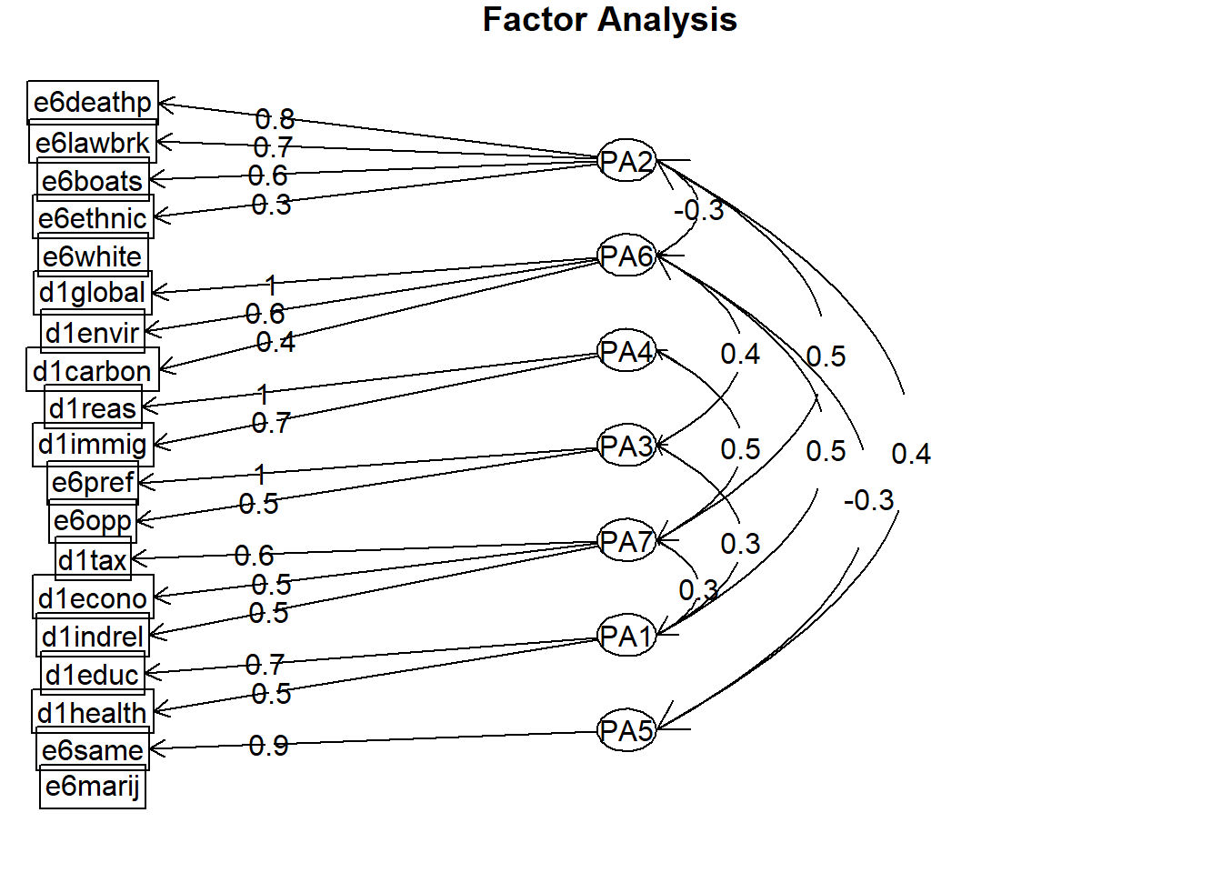
Visualise
fa.diagram(results.1)
Seven Factor Solution: Orthogonal (varimax rotation)
Run analysis
results.2 <- fa(r = attitudes, nfactors = 7, rotate = "varimax", fm="pa")
## maximum iteration exceeded
results.2
## Factor Analysis using method =  pa
## Call: fa(r = attitudes, nfactors = 7, rotate = "varimax", fm = "pa")
## Standardized loadings (pattern matrix) based upon correlation matrix
##            PA2   PA6   PA4   PA3   PA1   PA7   PA5   h2   u2 com
## d1tax     0.18  0.00  0.04  0.02  0.09  0.52  0.04 0.32 0.68 1.3
## d1immig   0.18  0.05  0.65 -0.01  0.14  0.24  0.06 0.53 0.47 1.6
## d1educ   -0.06  0.14  0.11  0.12  0.69  0.21 -0.03 0.56 0.44 1.4
## d1envir  -0.16  0.57  0.08  0.14  0.42  0.08 -0.15 0.58 0.42 2.5
## d1indrel  0.06  0.16  0.11  0.04  0.22  0.46  0.03 0.30 0.70 1.9
## d1health  0.09  0.12  0.10  0.08  0.55  0.29  0.02 0.42 0.58 1.8
## d1reas    0.00  0.14  0.88 -0.01  0.08  0.06  0.03 0.80 0.20 1.1
## d1global -0.18  0.86  0.07  0.15  0.21  0.03 -0.17 0.86 0.14 1.4
## d1carbon -0.03  0.39  0.21  0.04 -0.01  0.32 -0.01 0.30 0.70 2.6
## d1econo   0.15  0.02  0.08 -0.08  0.14  0.50  0.09 0.31 0.69 1.6
## e6deathp  0.72 -0.06  0.01  0.10  0.00  0.09  0.08 0.54 0.46 1.1
## e6marij  -0.14  0.10 -0.02  0.09 -0.02 -0.05 -0.27 0.11 0.89 2.2
## e6lawbrk  0.64 -0.03  0.02  0.01  0.09  0.08  0.09 0.44 0.56 1.1
## e6pref    0.07  0.03 -0.01  0.89 -0.01  0.06 -0.01 0.80 0.20 1.0
## e6boats   0.67 -0.15  0.11  0.02 -0.11  0.16  0.23 0.57 0.43 1.6
## e6same    0.22 -0.07  0.06  0.03 -0.07  0.07  0.86 0.81 0.19 1.2
## e6white  -0.22  0.06 -0.02  0.22  0.05 -0.08  0.07 0.12 0.88 2.8
## e6ethnic  0.34 -0.03  0.04 -0.11  0.00  0.09  0.13 0.16 0.84 1.7
## e6opp    -0.03  0.12  0.01  0.48  0.18 -0.01 -0.12 0.29 0.71 1.6
##
##                        PA2  PA6  PA4  PA3  PA1  PA7  PA5
## SS loadings           1.77 1.34 1.31 1.17 1.15 1.09 0.99
## Proportion Var        0.09 0.07 0.07 0.06 0.06 0.06 0.05
## Cumulative Var        0.09 0.16 0.23 0.29 0.35 0.41 0.46
## Proportion Explained  0.20 0.15 0.15 0.13 0.13 0.12 0.11
## Cumulative Proportion 0.20 0.35 0.50 0.63 0.76 0.89 1.00
##
## Mean item complexity =  1.7
## Test of the hypothesis that 7 factors are sufficient.
##
## The degrees of freedom for the null model are  171  and the objective function was  4.21 with Chi Square of  16628
## The degrees of freedom for the model are 59  and the objective function was  0.09
##
## The root mean square of the residuals (RMSR) is  0.01
## The df corrected root mean square of the residuals is  0.02
##
## The harmonic number of observations is  3780 with the empirical chi square  266.91  with prob <  3.2e-28
## The total number of observations was  3955  with Likelihood Chi Square =  372.41  with prob <  4.8e-47
##
## Tucker Lewis Index of factoring reliability =  0.945
## RMSEA index =  0.037  and the 90 % confidence intervals are  0.033 0.04
## BIC =  -116.27
## Fit based upon off diagonal values = 0.99
## Measures of factor score adequacy
##                                                    PA2  PA6  PA4  PA3  PA1
## Correlation of (regression) scores with factors   0.85 0.90 0.90 0.90 0.78
## Multiple R square of scores with factors          0.72 0.81 0.81 0.81 0.60
## Minimum correlation of possible factor scores     0.44 0.61 0.63 0.62 0.21
##                                                    PA7  PA5
## Correlation of (regression) scores with factors   0.72 0.88
## Multiple R square of scores with factors          0.52 0.77
## Minimum correlation of possible factor scores     0.04 0.55
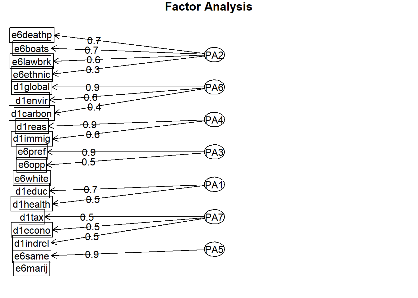
Visualise
fa.diagram(results.2)
Three factor solution: Oblique (promax rotation)
Run analysis
results.3 <- fa(r = attitudes, nfactors = 3, rotate = "promax", fm="pa")
results.3
## Factor Analysis using method =  pa
## Call: fa(r = attitudes, nfactors = 3, rotate = "promax", fm = "pa")
## Standardized loadings (pattern matrix) based upon correlation matrix
##            PA2   PA1   PA3    h2   u2 com
## d1tax     0.27  0.31  0.03 0.184 0.82 2.0
## d1immig   0.15  0.59 -0.21 0.407 0.59 1.4
## d1educ   -0.09  0.51  0.18 0.339 0.66 1.3
## d1envir  -0.37  0.55  0.23 0.553 0.45 2.1
## d1indrel  0.09  0.47  0.05 0.243 0.76 1.1
## d1health  0.09  0.49  0.17 0.304 0.70 1.3
## d1reas   -0.05  0.55 -0.24 0.291 0.71 1.4
## d1global -0.43  0.49  0.21 0.536 0.46 2.3
## d1carbon -0.10  0.46 -0.03 0.200 0.80 1.1
## d1econo   0.22  0.37 -0.07 0.209 0.79 1.7
## e6deathp  0.74 -0.03  0.30 0.465 0.53 1.3
## e6marij  -0.24  0.00  0.09 0.082 0.92 1.3
## e6lawbrk  0.63  0.04  0.20 0.356 0.64 1.2
## e6pref    0.24 -0.06  0.66 0.355 0.65 1.3
## e6boats   0.80 -0.03  0.12 0.584 0.42 1.0
## e6same    0.47 -0.02 -0.03 0.231 0.77 1.0
## e6white  -0.14 -0.04  0.19 0.074 0.93 1.9
## e6ethnic  0.36  0.05 -0.04 0.143 0.86 1.1
## e6opp     0.05  0.03  0.58 0.330 0.67 1.0
##
##                        PA2  PA1  PA3
## SS loadings           2.42 2.35 1.11
## Proportion Var        0.13 0.12 0.06
## Cumulative Var        0.13 0.25 0.31
## Proportion Explained  0.41 0.40 0.19
## Cumulative Proportion 0.41 0.81 1.00
##
##  With factor correlations of
##       PA2  PA1   PA3
## PA2  1.00 0.11 -0.38
## PA1  0.11 1.00  0.21
## PA3 -0.38 0.21  1.00
##
## Mean item complexity =  1.4
## Test of the hypothesis that 3 factors are sufficient.
##
## The degrees of freedom for the null model are  171  and the objective function was  4.21 with Chi Square of  16628
## The degrees of freedom for the model are 117  and the objective function was  0.88
##
## The root mean square of the residuals (RMSR) is  0.05
## The df corrected root mean square of the residuals is  0.06
##
## The harmonic number of observations is  3780 with the empirical chi square  3216.5  with prob <  0
## The total number of observations was  3955  with Likelihood Chi Square =  3484.7  with prob <  0
##
## Tucker Lewis Index of factoring reliability =  0.701
## RMSEA index =  0.085  and the 90 % confidence intervals are  0.083 0.088
## BIC =  2515.6
## Fit based upon off diagonal values = 0.93
## Measures of factor score adequacy
##                                                    PA2  PA1  PA3
## Correlation of (regression) scores with factors   0.90 0.89 0.82
## Multiple R square of scores with factors          0.82 0.79 0.66
## Minimum correlation of possible factor scores     0.63 0.58 0.33
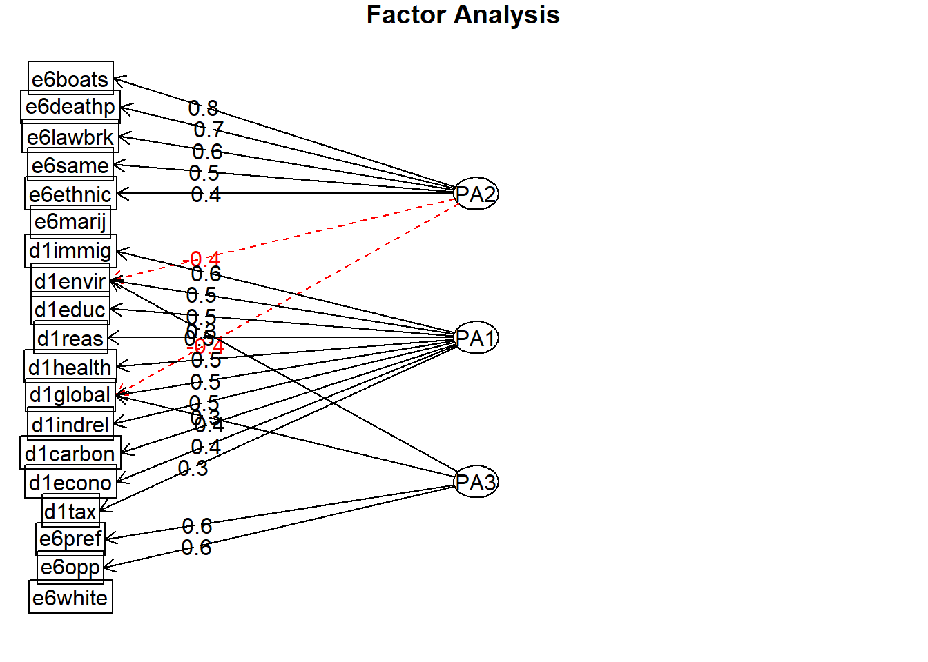
Visualise
fa.diagram(results.3)
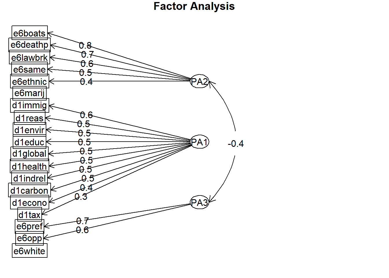
Three factor solution: Orthogonal (varimax rotation)
Run analysis
results.4 <- fa(r = attitudes, nfactors = 3, rotate = "varimax", fm="pa")
results.4
## Factor Analysis using method =  pa
## Call: fa(r = attitudes, nfactors = 3, rotate = "varimax", fm = "pa")
## Standardized loadings (pattern matrix) based upon correlation matrix
##            PA2   PA1   PA3    h2   u2 com
## d1tax     0.28  0.33  0.02 0.184 0.82 2.0
## d1immig   0.24  0.57 -0.17 0.407 0.59 1.5
## d1educ   -0.09  0.52  0.24 0.339 0.66 1.5
## d1envir  -0.37  0.55  0.33 0.553 0.45 2.5
## d1indrel  0.11  0.47  0.08 0.243 0.76 1.2
## d1health  0.08  0.51  0.20 0.304 0.70 1.4
## d1reas    0.04  0.51 -0.17 0.291 0.71 1.2
## d1global -0.43  0.49  0.32 0.536 0.46 2.7
## d1carbon -0.05  0.44  0.03 0.200 0.80 1.0
## d1econo   0.26  0.37 -0.07 0.209 0.79 1.9
## e6deathp  0.66  0.05  0.16 0.465 0.53 1.1
## e6marij  -0.26 -0.01  0.12 0.082 0.92 1.4
## e6lawbrk  0.58  0.10  0.09 0.356 0.64 1.1
## e6pref    0.08  0.04  0.59 0.355 0.65 1.0
## e6boats   0.76  0.04 -0.02 0.584 0.42 1.0
## e6same    0.47  0.00 -0.11 0.231 0.77 1.1
## e6white  -0.18 -0.02  0.20 0.074 0.93 2.0
## e6ethnic  0.36  0.07 -0.09 0.143 0.86 1.2
## e6opp    -0.08  0.11  0.56 0.330 0.67 1.1
##
##                        PA2  PA1  PA3
## SS loadings           2.38 2.35 1.15
## Proportion Var        0.13 0.12 0.06
## Cumulative Var        0.13 0.25 0.31
## Proportion Explained  0.40 0.40 0.20
## Cumulative Proportion 0.40 0.80 1.00
##
## Mean item complexity =  1.5
## Test of the hypothesis that 3 factors are sufficient.
##
## The degrees of freedom for the null model are  171  and the objective function was  4.21 with Chi Square of  16628
## The degrees of freedom for the model are 117  and the objective function was  0.88
##
## The root mean square of the residuals (RMSR) is  0.05
## The df corrected root mean square of the residuals is  0.06
##
## The harmonic number of observations is  3780 with the empirical chi square  3216.5  with prob <  0
## The total number of observations was  3955  with Likelihood Chi Square =  3484.7  with prob <  0
##
## Tucker Lewis Index of factoring reliability =  0.701
## RMSEA index =  0.085  and the 90 % confidence intervals are  0.083 0.088
## BIC =  2515.6
## Fit based upon off diagonal values = 0.93
## Measures of factor score adequacy
##                                                    PA2  PA1  PA3
## Correlation of (regression) scores with factors   0.90 0.88 0.78
## Multiple R square of scores with factors          0.81 0.77 0.62
## Minimum correlation of possible factor scores     0.62 0.55 0.23