2012 AuSSA data
Workshop 3 introduces the 2012 Australian Survey of Social Attitudes (AuSSA). AuSSA is a longitudinal survey (but it is a repeated cross-sectional survey, not a panel survey.) about social attitudes, beliefs and opinions of Australians. It is a biennial survey that began in 2003. It has been the main source of data for studies about how Australians think and feel about their lives as well as about how they have changed over time. AuSSA is also the Australian component of the International Social Survey Programme (ISSP). The ISSP is a cross-national collaboration on surveys covering important topics for social science research (If you want to know more about it, visit here). In addition, the ISSP chooses a special topic each year, which is called a module and repeats that topic from time to time. The module topic for 2012 was Family and Changing Gender Roles. The 2012 AuSSA is the most recent ISSP data on this topic.
In this workshop, we will use this dataset. The dataset is extracted from the 2012 ISSP data but includes only Australian respondents. This 2012 AuSSA is one of the datasets that you will use for the final data analysis report. If you want to know more about the 2012 AuSSA, visit https://www.acspri.org.au/aussa/2012.
How to open the 2012 AuSSA in SPSS
The dataset is not publicly available. I get the permission of using this dataset just for educational purposes. Therefore, use this dataset only for this unit.
Go to the course iLearn page and find The 2012 AuSSA SPSS Data File under the section of Datasets. Download this file. The downloaded data file should be aussa2012.sav. If you completed Preparation for the Workshops, this data file is already in your SSCI2020 folder at AppStream. Also, download and look at A Simple Codebook of the 2012 AuSSA and A Detailed Codebook of the 2012 AuSSA which all provide useful information on variables and their values in the dataset.
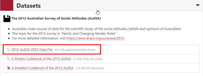
Figure 1: <Figure 1>
Open SPSS and follow the below steps.
- Go to File > Open > Data.
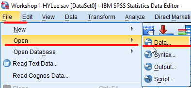
Figure 2: <Figure 2>
- In the window of Open Data, go to the SSCI2020 folder (Google Drive >> My Drive >> SSCI2020). Choose “aussa2012.sav” and click Open.
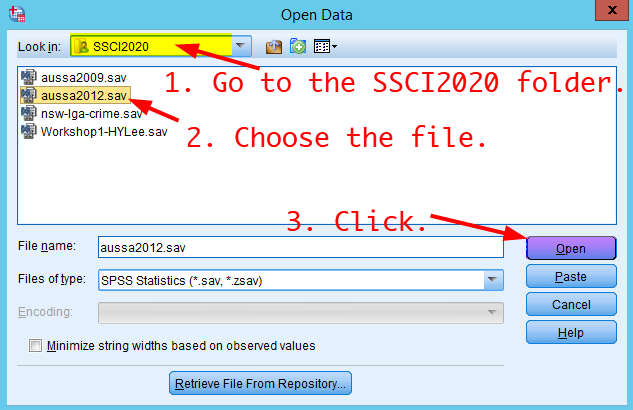
Figure 3: <Figure 3>
Troubleshooting: If you don’t see “aussa2012.sav” file in your SSCI2020 folder, Please follow the instruction at How to Upload Data Files.
Exploring the 2012 AuSSA
Click Variable View at the bottom. You will see the information on all the variables. Note that the level of measurement for all variables is not correctly specified: they are all Scales. Thus, you NEED TO ASSIGN appropriate levels of measurement for all the variables you will analyse before you start an analysis.
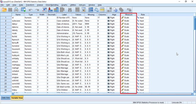
Figure 4: <Figure 4>
For example, suppose that we are analysing a variable, fepresch. To obtain detailed information on this variable, open “A Detailed Codebook of the 2012 AuSSA” using Adobe Acrobat Reader (You can download it here). Click the icon of Bookmark in the left pane.
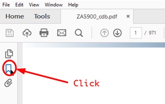
Figure 5: <Figure 5>
You will see the variable list in the left pane. Click the variable you want to study. In this example, the variable is fepresch. Then, the pdf will show the page which explains the variable of your choice.
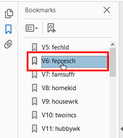
Figure 6: <Figure 6>
The codebook shows the questionnaire and response options, which helps you to figure out the level of measurement for variables.
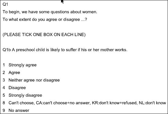
Figure 7: <Figure 7>
<Figure 7> shows the information on fepresch. It asks respondents the extent to which they agree or disagree with the statement that a preschool child is likely to suffer if his or her mother works. Although you see nine response options, we will take into account only five options (Strongly agree; Agree; Neither agree nor disagree; Disagree; Strongly disagree) as valid options. The other two options (Can’t choose; No answer) will be counted as system missing values, which will be explained in the next section. Because the five response options can be rank-ordered but do not have the same distance between them, fepresch is an ordinal variable. Change the level of measurement for fepresch. If you don’t remember how to do that, see Entering political orientation variable (ordinal variable).
I recommend you spend some time looking around variables in the 2012 AuSSA. The dataset includes so many variables relating to gender and family issues. You may find many variables that inspire your intellectual curiosity. In the final data analysis report, you need to find variables for your research project. Skim over all the variables in the codebook. This will also help you to find the topic of your final data analysis report.
Missing values
Missing or invalid values are generally too common to ignore. Survey respondents may refuse to answer specific questions, may not know the answer, or may respond in an unexpected format. If you include these kinds of invalid responses in your analysis, your analysis will provide inaccurate results.
For numeric data, empty data fields or fields containing invalid entries are converted to system-missing, which is identifiable by a single period(.). But more common practice is that some numerical values are treated as missing values. For example, in <Figure 7>, 8 denotes “Can’t choose”, and 9 represents “No answer”. These responses are typical types of missing values. In Variable View, click a small square in the column of Missing for fepresch (see <Figure 8>). You will see that 0, 8 and 9 are treated as missing values in the popped-up window (see <Figure 9>). To be back to the previous Variable View tab, click OK in the popped-up window.
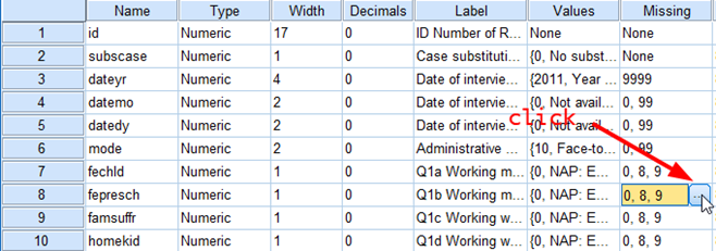
Figure 8: <Figure 8>
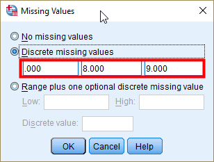
Figure 9: <Figure 9>
When analysing variables SPSS always show the number of missing values, but does not take into account them when calculating statistics(e.g., mean, median, standard deviation). For example, look at the frequency table of fepresch in <Figure 10>. You will see the frequency of two missing categories (8 = Can’t choose; 9 = No answer) in the bottom. 19 respondents chose “Can’t choose”, and 38 respondents didn’t provide answers. Thus, the number of missing cases is 57(19+38), which is 3.5% of the total number of cases (See <Figure 10>). Also, note that the Percent in the table is based on all responses, including missing values, while the Valid Percent is based on only valid responses which exclude missing values. Your next question might be which percent (more broadly, which statistics) you should report. My recommendation is to report the valid percent because we usually are interested only in valid responses.
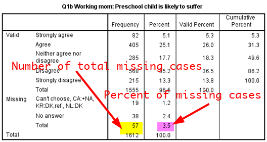
Figure 10: <Figure 10>
Workshop 3 Participation Activity |
(1) A nominal variable
(2) An ordinal variable (3) A continuous variable (4) Can’t identify
|
NOTE: After you get the outcome of statistical analysis in the Output window, DO NOT close the Output window to go back to Data Editor. Instead, use the icon of Switch windows on the top menu of AppStream. For more details, see Switch windows. Keep the Output window open. All your statistical outcomes will be stored in the Output window. Then, you will be able to export them to other documents. The last section of this workshop will introduce how to export your statistical outcomes.
Descriptive Statistics
This section introduces how to compute descriptive statistics. fepresch (ordinal variable) and age (continuous variable) are used for this task. Please assign correct levels of measurements for these two variables before you start the analysis.
Computing descriptive statistics using Explore
Go to Analyze > Descriptive Statistics > Explore. In the window of Explore, select variables for which you want to compute descriptive statistics (in this example, they are fepresch and age) and move them into the pane of Dependent List. Click Plots.
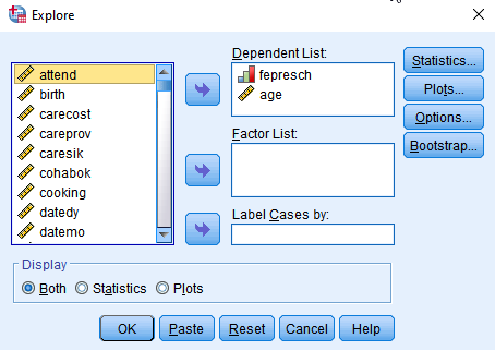
Figure 11: <Figure 11>
Troubleshooting: If you see variable labels instead of variable names, right-click at the left variable pane. Choose Display Variable Names. You will see variable names instead of variable labels. Also, choose Sort Alphabetically. Then, variables will be listed in an alphabetical order, which may make it easier to locate a variable of your interest. For more details, see the second step of Making a frequency table.
In the window of Explore: Plots, tick only Histogram in the section of Descriptive. The histogram is for age which is a continuous variable. Click Continue. You will be back to the previous window. Then, click OK at the bottom.
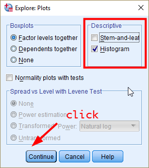
Figure 12: <Figure 12>
In the output window, you will see the descriptive statistics of both fepresch and age (see <Figure 13>). First, look at Case Processing Summary. You can see how many respondents provide valid and missing responses in each variable. In both fepresch and age, 104 respondents provide missing(invalid) responses, which is 6.5% of the total number of cases. Therefore, 93.5% (You can find this percent in Percent of Valid.) of respondents in the sample provide valid responses in these two variables.
Then, look at Descriptives. The output shows almost all descriptive statistics. You can find two measures of central tendency (mean and median) and four measures of variability(variance, std. deviation, range, interquartile range). Also, skewness scores are reported so that you can adjudicate the skewness of distributions. Moreover, the visualisation of variables (e.g., histograms and box plots) is shown as well. Therefore, Explore command is a handy way to see the distribution of ordinal or continuous variables.
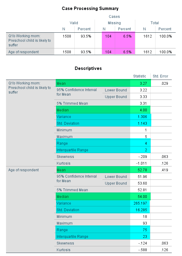
Figure 13: <Figure 13>
Based on <Figure 13>, which measure of central tendency describes best the distribution of fepresch? Recall what you learned from the week 4 lecture. fepresch is an ordinal variable. Thus, the median best represents the central tendency of the distribution for ordinal variables. Therefore, to describe the central tendency of fepresch, you can say that “Disagree”(which corresponds to the median value 4) is the median response to whether people agree or disagree to the statement that a preschool child is likely to suffer if his or her mother works.
Based on <Figure 13>, which measure of central tendency describes best the distribution of age? age is a continuous variable. Thus, you need to check the skewness of the distribution first. The skewness score is -0.124, which falls on the acceptable range (-0.5 ≤ skewness ≤ 0.5). Thus, we can say that the distribution of age is approximately normal. Consequently, the best measure of central tendency for age distribution is a mean, which is 52.78.
Workshop 3 Participation Activity |
(1) 2
(2) 37.52 (3) 40 (4) 96 |
Comparing descriptive statistics between groups using Explore
Another advantage of using Explore is that it allows you to compare descriptive statistics between groups. Suppose that we want to compare the age of respondents between men and women. Thus, we need to compute the measures of central tendency and variability for men and women respectively so that we can compare these measures between them.
Go to Analyze > Descriptive Statistics > Explore. In the window of Explore, click Reset at the bottom to remove the variables you used before. Then, 1) select variables for which you want to compute descriptive statistics (in this example, it is age) and move it to the pane of Dependent List. 2) select a group variable (in this example, it is sex) by which descriptive statistics are compared and move it to the pane of Factor List. Make sure that a group variable should be either a nominal or ordinal variable. See the icon of sex variable in <Figure 14>. The three circles indicate nominal variables. Click Plots. As you did in <Figure 12>, tick only Histogram in the window of Explore: Plots. Click Continue. You will be back to the previous window. Then, click OK at the bottom.
Troubleshooting: If the icon of sex variable is not three circles, you need to change the level of measurement for sex. Click Variable View at the bottom. Then, find sex variable. Change measures from Scale to Nominal, and save the data. If you are not sure how to do it, see Entering gender variable in the workshop 1 instruction.
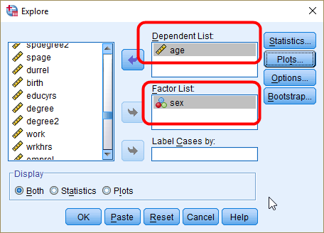
Figure 14: <Figure 14>
In the output window, you will see the descriptive statistics for both men and women. (see <Figure 15>). Also, you will see the box plot of age by gender, which is very helpful for comparing the distribution between men and women (see <Figure 16>). If you are not sure how to read box plots, review the week 4 lecture slides.
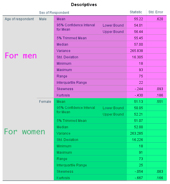
Figure 15: <Figure 15>
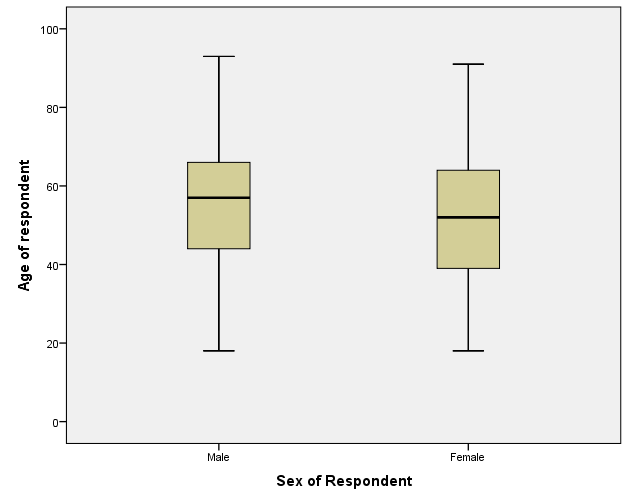
Figure 16: <Figure 16>
Workshop 3 Participation Activity |
|
Creating another copy of datasets.
So far, you have assigned appropriate levels of measurement to several variables. Thus, the dataset on which you are working should be different from the one you opened at the beginning of this workshop. As a result, I recommend you to create another copy of “aussa2012.sav”. In the Data Editor(Make sure that it should be Data Editor window, not Output), go to File > Save as.
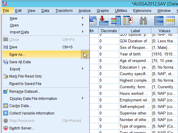
Figure 17: <Figure 17>
In the box of Save Data As, 1) choose the SSCI2020 folder in the section of Look in, 2) choose “SPSS Statistics (.sav)” in Save as type, 3) type file names (use names different from “aussa2012.sav”. In the example, I use “aussa2012-1.sav”), and 4) click Save. Your file will be saved in the SSCI2020 folder.
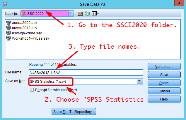
Figure 18: <Figure 18>
Saving SPSS outputs
Now, I would like to introduce how to save all your output in the same document. I assume that you didn’t close the SPSS Output window so far. Thus, your output window should include all the outcomes of the workshop 3.
You have two options to save your SPSS outputs that you have created so far. The first option is to save them as the format of “SPSS viewers (.spv)”. This format saves your SPSS outputs in the same way as you see in the Output window. Thus, it is the best way to save your SPSS outputs. However, you can open this format only in SPSS. This means that you have to log on AppStream to open this format of files. The second option is to save your SPSS outputs as the format of “SPSS Web Report (.htm)”. The advantage of this format is that you can open this format of files with your web browser. So, you need not log on AppStream to see your SPSS outputs. However, the display of outputs looks a little bit different from what you see in the Output window. As a result, my recommendation is to save your SPSS outputs in both ways. You will be able to take advantage of both formats.
Option 1: SPSS Viewer Format (.spv)
- In the window of Output (Make sure that it should be Output window, not Data Editor), go to File > Save.
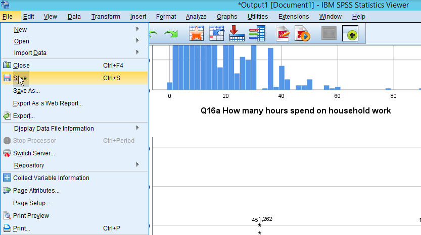
Figure 19: <Figure 19>
- In the window of Save Output As, 1) choose the folder of SSCI2020 in the section of Look in, 2) type file names, 3) choose Viewer Files (.spv) in Save as type, and 4) click Save. Your file will be saved in the SSCI2020 folder.
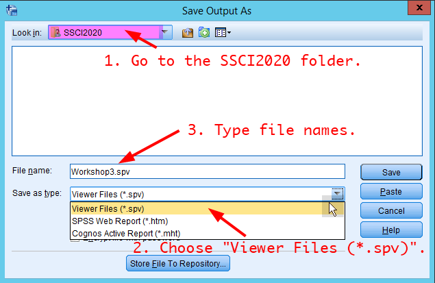
Figure 20: <Figure 20>
Now, I would like to show how to open this saved SPSS viewer files.
- Close the Output window.
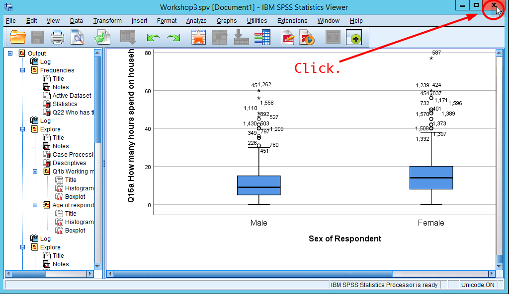
Figure 21: <Figure 21>
- In either Data Editor or Output window, go to File > Open > Output.
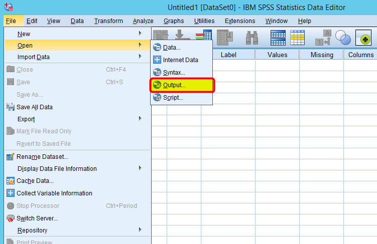
Figure 22: <Figure 22>
- In the window of Open Output, 1) choose the folder of SSCI2020 in the section of Look in, 2) choose the file where you saved the output. In this example, the file is “Workshop3.spv”. and 3) click Open. You will see the SPSS output you saved before.
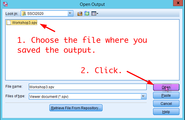
Figure 23: <Figure 23>
Option 2: HTML Format (.htm)
- In the window of Output(Make sure that it should be Output window, not Data Editor), go to File > Export.
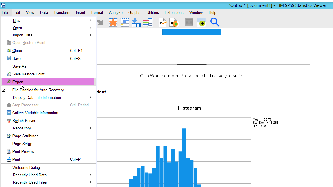
Figure 24: <Figure 24>
- In the window of Export Output, 1) choose **“HTML (*.htm)“** as the type of document , and then 2) click Browse (See <Figure 25>).
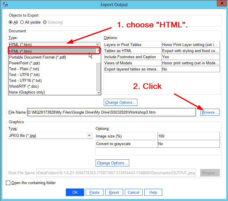
Figure 25: <Figure 25>
- choose the folder of SSCI2020 in the section of Look in, 2) type file names, 3) choose HTML (.htm) in Save as type, and 4) click Save.
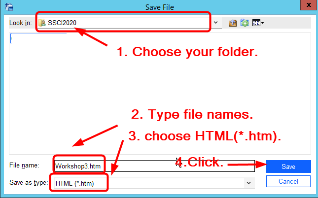
Figure 26: <Figure 26>
You will be back to <Figure 25>. Click OK at the bottom. Your file will be saved in the SSCI2020 folder.
Next, you need to download the saved HTML file from AppStream. Click the icon of My Files in the AppStream navigation bar (See <Figure 27>). Go to SSCI2020 folder. You will see the saved file (in this example, it is Workshop3.htm). Click the name of this file. It will be downloaded (See <Figure 28>).

Figure 27: <Figure 27>
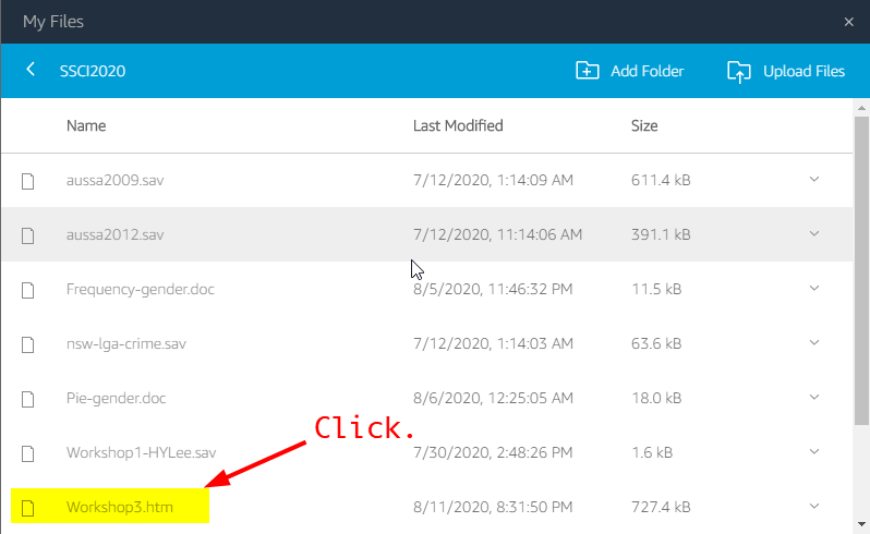
Figure 28: <Figure 28>
- Open the downloaded file in your local computer. In most cases, you can find the file in your Download folder. You will see your saved outputs in your web browser (See <Figure 29>). You can copy any outputs in this HTML file and paste them to other documents.
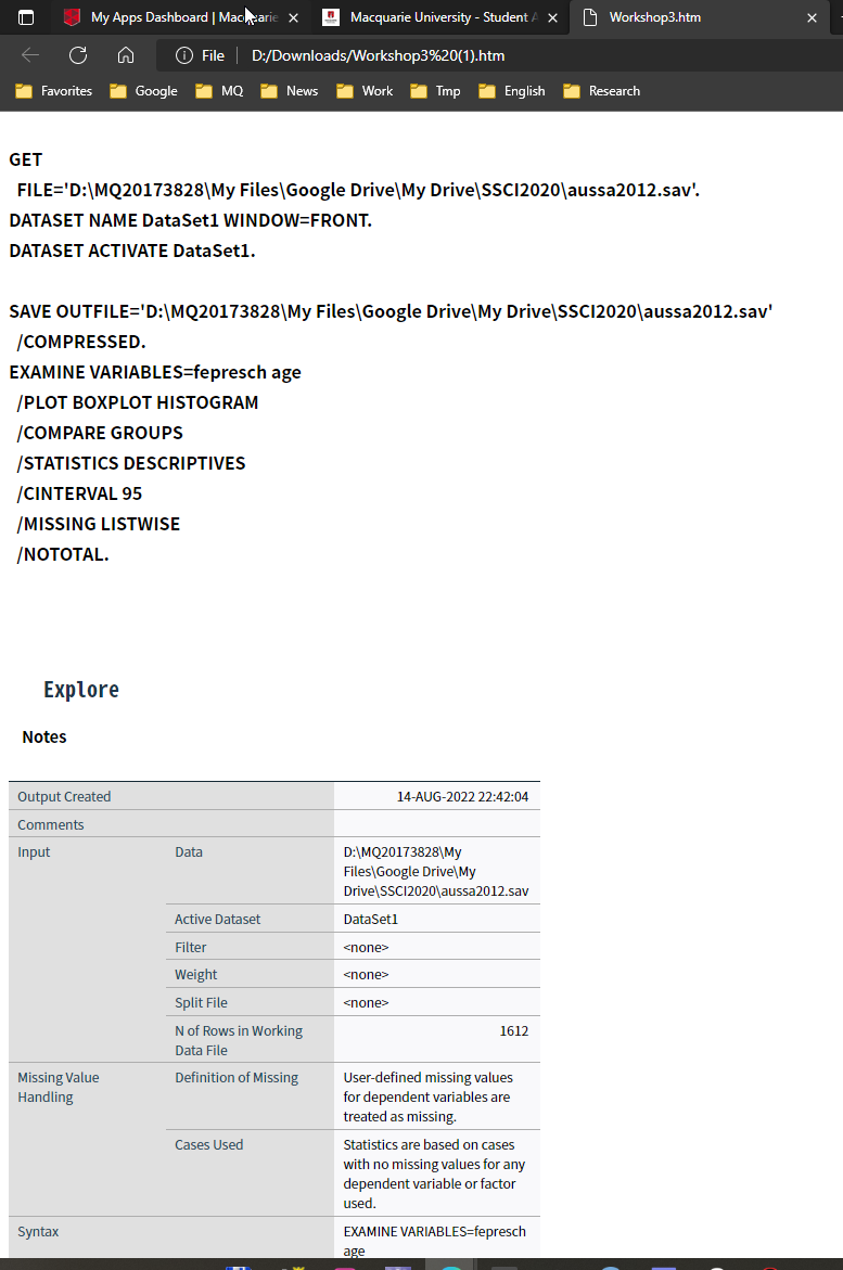
Figure 29: <Figure 29>