In workshop 11, we will learn the regression analysis, a powerful statistical model that enables you to examine the effect of independent variables on the dependent variable. We continue using the NSW Crime Dataset.Please open it.
Preparation
Selecting Cases of Complete Observations
In most cases, your dataset contains cases with many missing values. Missing values can reduce the statistical power of analyses and produce biased estimates, which could lead to invalid conclusions. There are several ways to deal with missing values, but this workshop introduces only the method of “Listwise deletion” (also known as complete-case analysis) which is the most frequently used for handling missing data. You learned this method in workshop 10 when you created the correlation matrix. But this workshop introduces a more general way that can be used for all kinds of statistical analyses. You will learn how to select all the cases which have no missing values on the variables of your choice so that you can use these selected cases for any of your future analysis. Listwise deletion removes any case from the dataset if the case has a missing value on any variable of your choice. Suppose that we are investigating the relationships across five variables: sexual offence rates (sexoff), the median age of residents (medage), unemployment rates (unemploy), median house prices (housmedprice), and urban or rural LGAs (urban).
The first step of this analysis is to select all the LGAs that have no missing values on these six variables so that we can investigate all combinations of the relationships using the same set of LGAs. Go to Data > Select Cases (See <Figure 1>.
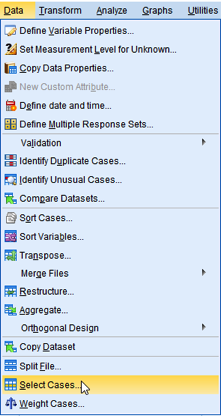
Figure 1: <Figure 1>
In the box of Select Cases, 1) choose “If condition is satisfied”. 2) In the section of Output, choose “Filter out unselected cases”, which will exclude unselected cases from the analysis. Then, 3) click the If just below “If condition is satisfied” in the section of Select (See <Figure 2>.
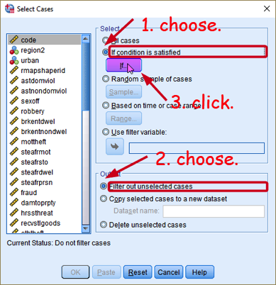
Figure 2: <Figure 2>
In the box of Select Cases: If, type the following expression (See <Figure 3>). You can copy and paste the below text into your SPSS.
NOT (SYSMIS(sexoff)) AND NOT (SYSMIS(medage)) AND NOT (SYSMIS(unemploy)) AND NOT (SYSMIS(housmedprice)) AND NOT (SYSMIS(urban))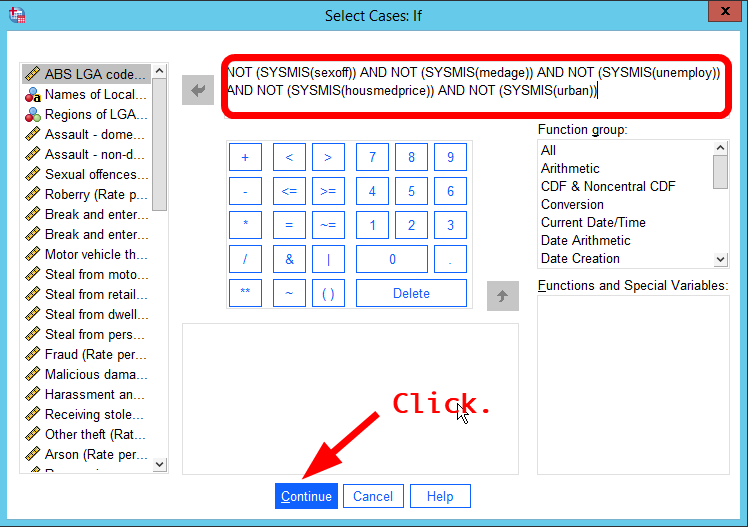
Figure 3: <Figure 3>
SYSMIS(variable) finds cases that have missing values on the variable. Thus, NOT SYSMIS(variable) finds cases that do not have missing values. AND signifies that all the listed conditions must be met. Combined together, the above expression will select cases that have no missing values on any of the six variables.
Click Continue at the bottom. Then, you will be back to the previous box. Click OK at the bottom. Make sure all the analysis after this point will be done only for the selected cases. Thus, if you want to analyse all the cases again, you need to deselect cases (See Deselecting cases).
Changing the Scale of Variables
housmedprice has a huge range (47500 – 2800000), which makes it a little bit complicated to interpret regression outputs. Therefore, reducing the range would be helpful. An easy way to achieve this goal is to divide the value by numbers. In this example, we divide it by 10,000.
Go to Transform > Compute Variable. In the box of Compute Variable, 1) type “housmedprice2”, which is a new variable name, in the section of Target Variable:, 2) click the icon of Type & Label, which will show the box of Compute Variable: Type and Label, 3) in the box, choose “Label”, type “Median Sale Price of Houses ($10,000)”, and click Continue, 4) type housmedprice/10000 in the section of Numeric Expression:, and 5) click OK at the bottom (see <Figure 4>).
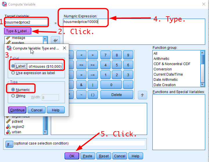
Figure 4: <Figure 4>
Simple Linear Regression
In this workshop, we will investigate what kinds of community characteristics influence sexual offence rates(sexoff). We start with a very simple version of regression model in which only the dependent variable is regressed on only one independent variable.
First, we will estimate the effect of the median sale price of houses (housmedprice2) on the sexual offence rate (sexoff). To conduct a linear regression analysis, go to Analyze > Regression > Linear (see <Figure 5>) .
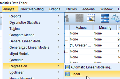
Figure 5: <Figure 5>
In the popped-up box of Linear Regression, 1) move sexoff to the section of Dependent, 2) move housmedprice2 to the section of Independent(s) and 3) click OK (see <Figure 6>).
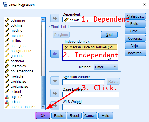
Figure 6: <Figure 6>
You will see the regression output as in <Figure 7>.
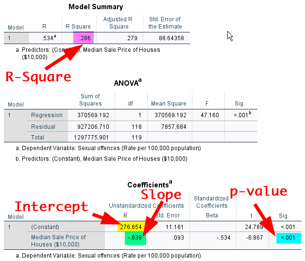
Figure 7: <Figure 7>
First, look at the table of Model Summary. You will see “R Square”. R Square (the coefficient of determination) tells you the proportion of the variance in the dependent variable explained by independent variables. In the table, R Square is .286, which means that 28.6% of the total variation in the sexual offence rate are explained by the median sale price of houses.
Second, look at the table of Coefficients. The intercept is 276.654. The coefficient (slope) of housmedprice2 is -.638, meaning that for each additional $10,000 in the median sale price of houses, sexual offence rates will decrease by .638. Therefore, the regression equation estimated by this model is \(sexoff = 276.654 -.638 × housmedprice2\).
Third, the table also provides the p-value for the significance test of the coefficient. The p-value for the coefficient of housmedprice2 is less than .001, indicating that the negative effect of housmedprice2 on sexoff is statistically significant at α = .05 (Note: We normally don’t pay attention to the p-value for intercepts).
Then, we will estimate the sexual offence rate by other two independent variables, respectively. In the box of Linear Regression (in <Figure 6>), move medage and unemploy to the section of Independent(s), respectively. You will get the regression output for medage (See <Figure 8>) and for unemploy (see <Figure 9>).
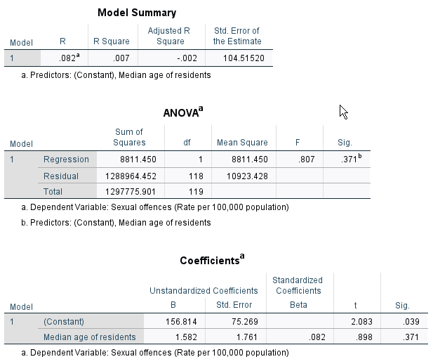
Figure 8: <Figure 8>
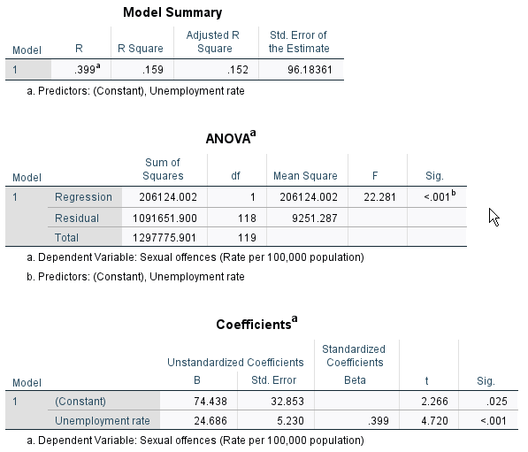
Figure 9: <Figure 9>
Multiple Regression
In this section, we will estimate the sexual offence rate by the three independent variables (housmedprice2, medage, unemploy) simultaneously. To conduct this multiple regression analysis, move all the three variables to the section of Independent(s) in the box of Linear Regression (See <Figure 10>)
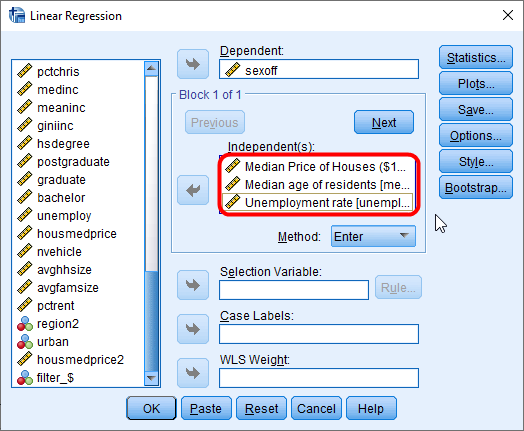
Figure 10: <Figure 10>
You will see the regression output as in <Figure 11>.
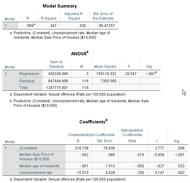
Figure 11: <Figure 11>
Again, focus on the table of Model Summary and Coefficient.
R Square is .347, which means that 34.7% of the total variance in the sexual offence rate are explained by the three variables.
The coefficient of housmedprice2 is -.562, meaning that for every additional $10,000 in the median sale price of house, sexual offence rates will decrease by .562, after controlling the median age of residents and unemployment rates. The p-value for this coefficent is less than .001, and thus the negative effect of housmedprice2 is statistically significant at α = .05.
The coefficient of medage is -.951, meaning that for each additional one year increase in the median age of respondents, sexual offence rates will decrease by .951, after controlling the median sale price of houses and unemployment rates. The p-value for this coefficent is .532, and thus the negative effect of medage is NOT statistically significant at α = .05.
The coefficient of unemploy is 15.510, meaning that for each additional 1% increase in the unemployment rate, sexual offence rates will increase by 15.510, after controlling the median sale price of houses and the median age of residents. The p-value for this coefficent is .002, and thus the positive effect of unemploy is statistically significant at α = .05.
The regression equation estimated by this model is \(sexoff = 216.738 -.562 × housmedprice2 -.951 × medage +15.51 × unemploy\).
Dummy Variable Analysis
Creating a Dummy Variable.
A dummy variable is a binary variable used in the regression analysis that represents subgroups (or categories) of the sample in your study. And it is used to estimate the effect of categorical (especially, nominal) variables. Suppose that we want to estimate the effect of regions on the sexual offence rate. More specifically, we want to compare this effect across three regions: Greater Metropolitan Sydney, Sydney Surrounds, and Rural and Regional Areas. Since this variable of regions is not a continuous variable (actually, it is a nominal variable), a set of dummy variables is necessary for estimating this effect.
Let’s make a set of dummy variables for the region. First, we need to recode region into region2, following the recoding scheme of <Table 1>.
| Values | Labels | Values | Labels |
|---|---|---|---|
| 1 | Greater Metropolitan Sydney | 1 | Greater Metropolitan Sydney |
| 2 | Sydney Surrounds | 2 | Sydney Surrounds |
| 3 | Mid North Coast | 3 | Rural and Regional Areas |
| 4 | Murray | ||
| 5 | Murrumbidgee | ||
| 6 | Hunter | ||
| 7 | Illawarra | ||
| 8 | Richmond-Tweed | ||
| 9 | Canberra Region | ||
| 10 | Northern | ||
| 11 | Central West | ||
| 12 | North Western | ||
| 13 | Far west |
After making region2, we need to make two dummy variables which represent “Sydney Surrounds” and “Rural and Regional Areas”, respectively (Note that when the nominal variable for which you want to estimate the effect has a N number of categories, you need to make a N-1 number of dummy variables). The omitted category in region2 (Greater Metropolitan Sydney) will serve as the reference category in estimating the effect of each region. Make a dummy variable for “Sydney Surrounds” (region2_d2), following the recoding scheme of <Table 2>. Note that values in a dummy variable take either 0 ( = not belong to the category) or 1 ( = belong to the category). Thus, 1 in the dummy variable for “Sydney Surrounds” indicates for an LGA in Sydney Surrounds.
| Values | Labels | Values | Labels |
|---|---|---|---|
| 1 | Greater Metropolitan Sydney | 0 | Else |
| 2 | Sydney Surrounds | 1 | Sydney Surrounds |
| 3 | Rural and Regional Areas | 0 | Else |
Also, make a dummy variable for “Rural and Regional Areas” (region2_d3), following the recoding scheme of <Table 3>.
| Values | Labels | Values | Labels |
|---|---|---|---|
| 1 | Greater Metropolitan Sydney | 0 | Else |
| 2 | Sydney Surrounds | 0 | Else |
| 3 | Rural and Regional Areas | 1 | Rural and Regional Areas |
Dummy Variable Regression Analysis
After making dummy variables, it is easy to estimate the effect of them. Move a set of dummy variables (in this example, region2_d2 and region2_d3) to the section of Independent(s) in the box of Linear Regression.
You will see the regression output as in <Figure 12>.
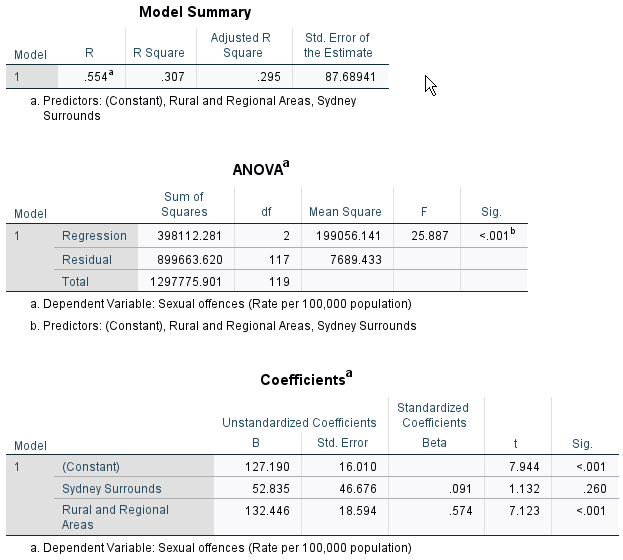
Figure 12: <Figure 12>
Notable results are:
R Square is .307, which means that 30.7% of the total variance in the sexual offence rate are explained by the set of two dummy variables of regions.
The coefficient of “Sydney Surrounds” is 52.835, meaning that LGAs in Sydney Surrounds have, on average, higher sexual offence rates than those in Greater Metropolitan Sydney by 52.835. However, this difference is not statistically significant at α = .05 (because the p-value (.260) is greater than α). Thus, we confirm that sexual offence rates do not differ significantly between Great Metropolitan Sydney and Sydney Surrounds.
The coefficient of “Rural and Regional Areas” is 132.446, meaning that LGAs in Rural and Regional Areas have, on average, higher sexual offence rates than those in Greater Metropolitan Sydney by 132.446. And this difference is statistically significant at α = .05 (because the p-value (<.001) is much less than α).
Then, we will examine whether these findings are consistent even after controlling community characteristics. In the box of Linear Regression, move region2_d2, region2_d3, housmedprice2, medage and unemploy to the section of Independent(s).
You will see the regression output as in <Figure 13>.
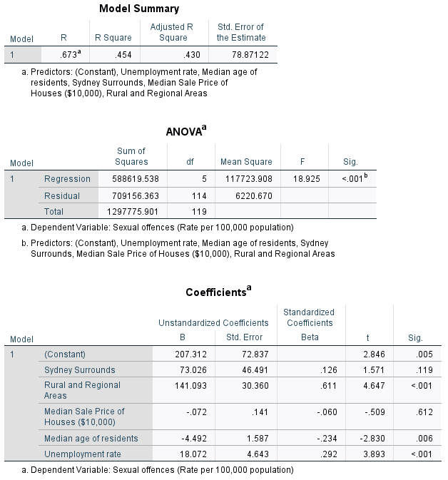
Figure 13: <Figure 13>
As seen in <Figure 13>, the findings in <Figure 12> are consistent even after controlling the median price of houses, the median age of residents, and unempoyment rates.
The coefficient of “Sydney Surrounds” is 73.026, but this coefficient is not statistically significant.
By contrast, the coefficient of “Rural and Regional Areas” is 141.093, meaning that LGAs in Rural and Regional Areas have, on average, higher sexual offence rates than those in Greater Metropolitan Sydney by 141.093 after controlling the median price of houses, the median age of residents, and unempoyment rates. And this difference is statistically significant at α = .05.
R Square is .454, which means that 45.4% of the total variance in the sexual offence rate are explained by all these five variables.
The regression equation estimated by this model is \(sexoff = 207.312 + 73.026 × region2\_d2 +141.093 × region2\_d3 -.072 × housmedprice2 -4.492 × medage +18.072 × unemploy\).
Workshop Activity 11: Regression Analysis |
|
For this workshop, you will conduct the regression analysis using a different set of cases. Please follow the steps below.
You are required to use this set of cases for Q1, Q2 and Q3.
|