In the workshop 8, we continue using the 2019 Australian Survey of Social Attitudes(2019 AuSSA). This workshop introduces how to estimate confidence intervals and how to conduct a t-test of sample means.
Compute Confidence Intervals
Confidence Intervals for Continuous Variables
Suppose that we want to estimate the 95% confidence intervals for Australians’ mean age using the 2019 AuSSA. To create a confidence interval, 1) go to Analyze > Descriptive Statistics > Explore. In the box of Explore, 2) select age (the variable should be a continuous variable) and move it to the box of Dependent List. 3) Click Statistics (See <Figure 1>).
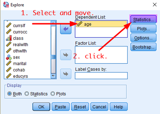
Figure 1: <Figure 1>
Then, in the box of Explore: Statistics, 4) tick Descriptives and 5) type a value of confidence level (in this case, 95) in the box of Confidence Interval for Mean. 6) Click Continue (See <Figure 2>).
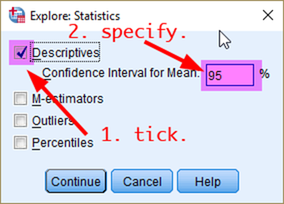
Figure 2: <Figure 2>
Now, you are back to the previous box. Click OK at the bottom. It will show the 95% confidence interval of Australians’ mean age (See <Figure 3>).
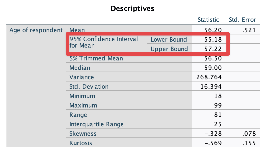
Figure 3: <Figure 3>
Confidence Intervals by Groups
Suppose that we want to estimate the 95% confidence intervals of Australians’ mean age for men and women, respectively. Go to Analyze > Descriptive Statistics > Explore. In the box of Explore, put age in the Dependent List and sex in the Factor List (see <Figure 4>). Note that the variable in the section of Dependent List should be a continuous variable, and the variable in the section of Factor List should be a nominal variable (Check the icon of variables, which shows the level of measurement).
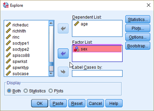
Figure 4: <Figure 4>
Click Statistics. Do the same thing as you did in the previous section. It will show the 95% confidence intervals of mean age for Australian men and women, respectively (see <Figure 5>).
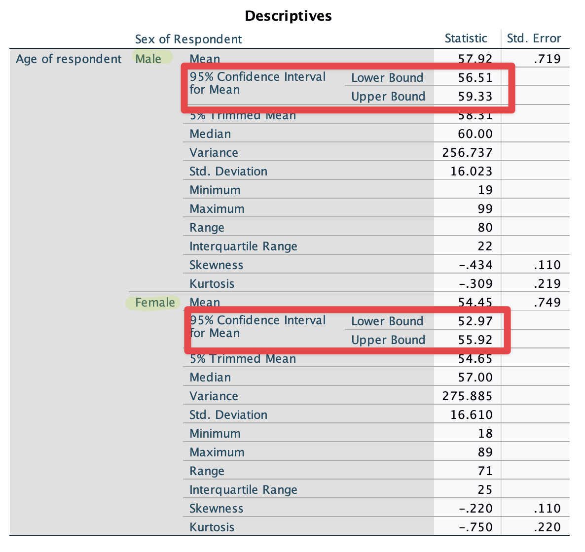
Figure 5: <Figure 5>
Confidence Intervals for Proportions
When you want to compute the confidence interval for a categorical (nominal or ordinal) variable, you first need to dichotomise the variable so that you can compute a proportion of a category. Suppose that we are estimating the 95% confidence interval for the proportion of people who think that it is important to come from a wealthy family (opwlth).
First, we need to dichotomise opwlth using Recode into Different Variables. <Table 1> shows the recoding scheme of the new dichotomised variable (newopwlth) Make this new variable (newopwlth) using opwlth.
| Values | Labels | Values | Labels |
|---|---|---|---|
| System- or user-missing | System- or user-missing | System-missing | System-missing |
| 1 | Essential | 1 | Important |
| 2 | Very important | ||
| 3 | Fairly important | ||
| 4 | Not very important | 0 | Not important |
| 5 | Not important at all |
Then, follow the same procedure as you did for getting the confidence interval for the mean age of Australians. <Figure 6> would be helpful.
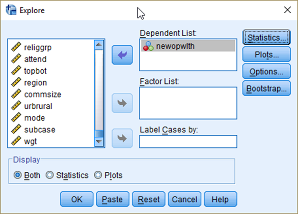
Figure 6: <Figure 6>
Then, you will see the ouput as in <Figure 7>.
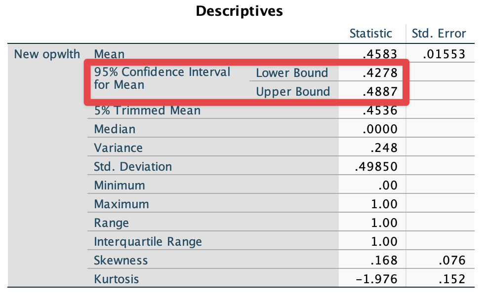
Figure 7: <Figure 7>
Now, we get the 95% confidence interval for the proportion of people who think that it is important to come from a wealthy family. But what if we want to get this proportion for men and women, respectively?
Put a variable of sex in the box of Factor List in <Figure 6>. Then, you will see <Figure 8>, which shows the 95% confidence intervals for the proportion for men and women, respectively.
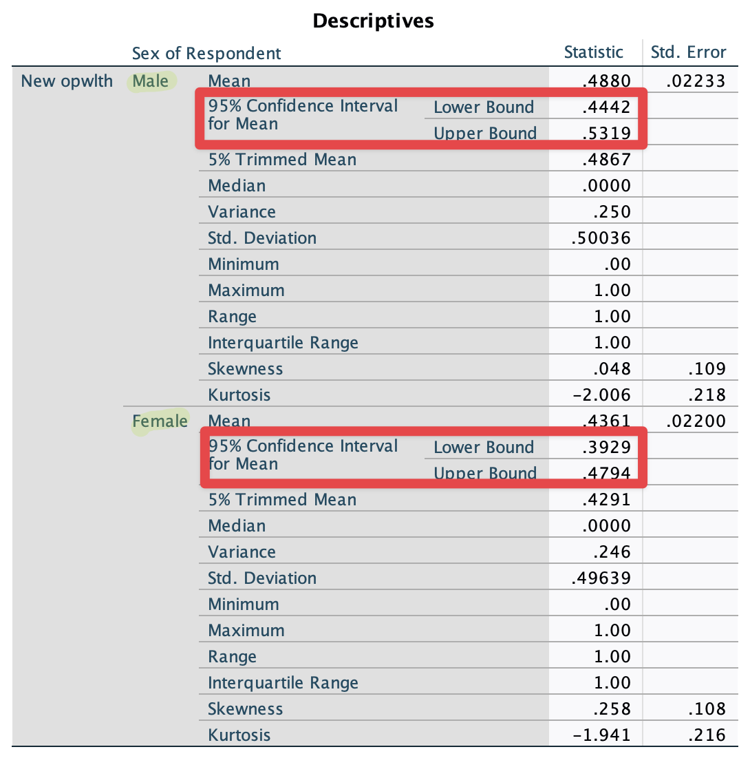
Figure 8: <Figure 8>
Visualising Confidence Intervals
Now, we are going to visualise the confidence intervals for the proportion of people who think that it is important to come from a wealthy family by gender. 1) Go to Graph > Error Bar. In the box of Error Bar, 2) select Simple and Summaries for groups of cases. 3) Click Define (see <Figure 9>).
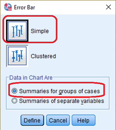
Figure 9: <Figure 9>
In the box of Define Simple Error Bar: Summaries for Groups of Cases , 4) move newopwlth to the section of Variable. 5) move sex in the section of Category Axis and then 6) Click OK (see <Figure 10>).
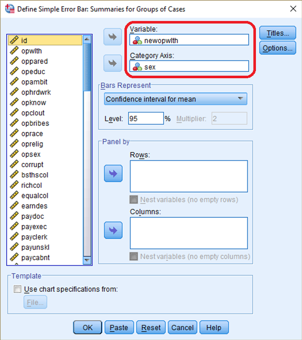
Figure 10: <Figure 10>
It will produce <Figure 11>. After looking at <Figure 11>, adjudicate whether men and women assess the importance of wealthy family backgrounds differently. If you are not sure how to do this, please see the week 8 lecture slides.
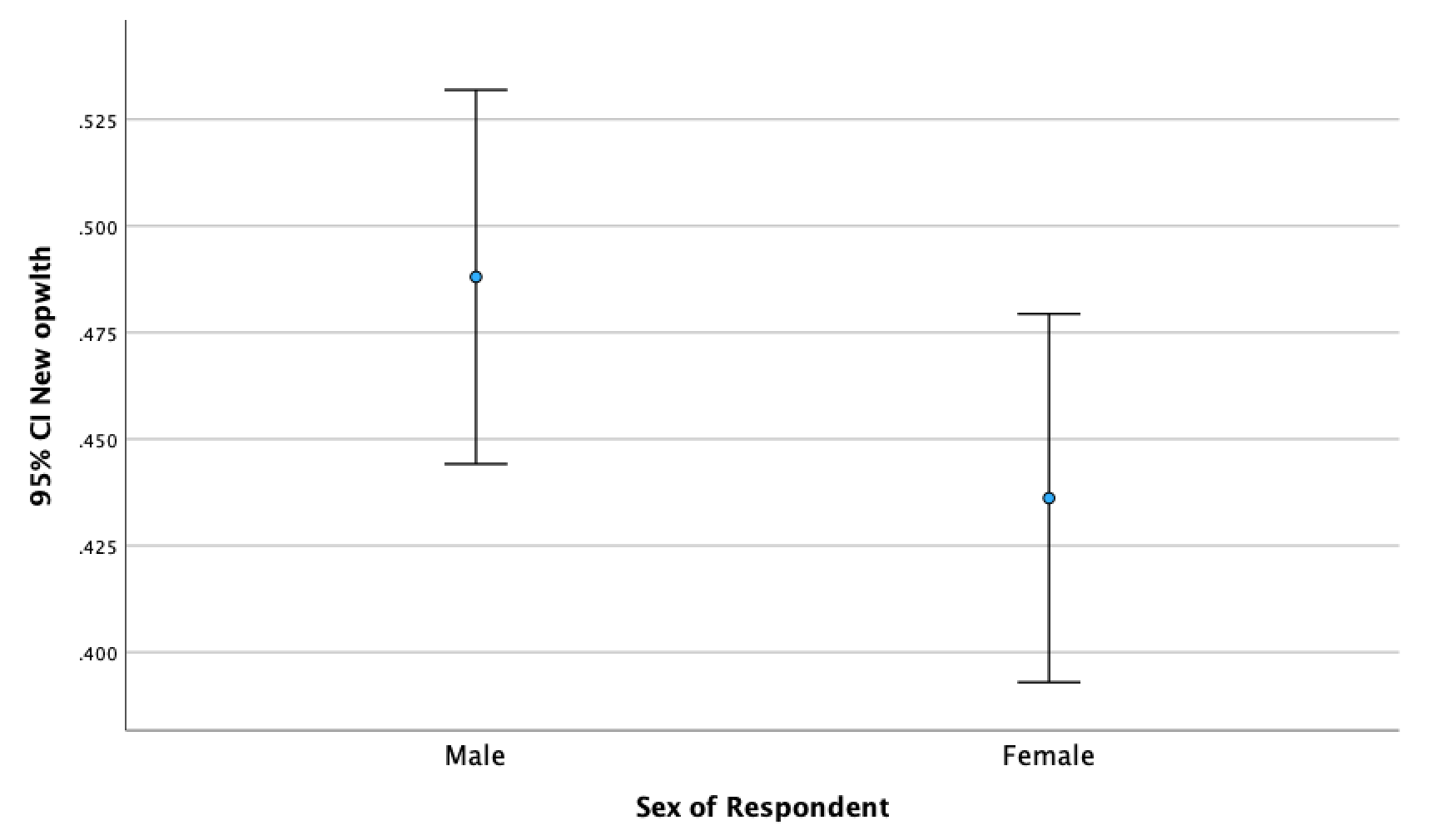
Figure 11: <Figure 11>
Hypothesis Testing
One-Sample t-Test
The standard working hours per week in Australia is currently 38. Let’s test whether Australians work, on average, 38 hours per week or not, using a variable, wrkhrs. We will test whether the average working hours of Australians is significantly different from 38 hours. Thus, our research hypothesis is that Australians work, on average, either more than or less than 38 hours per week. The null hypothesis is that Australians work, on average, 38 hours per week.
To conduct one-sample t-test, 1) go to Analyze > Compare Mean > One-Sample T Test. In the box of One-Sample T Test, 2) move a variable of your interest (in this case, wrkhrs) and 3) specify a test value which the null hypothesis assumes (in this case 38) (see <Figure 12>).
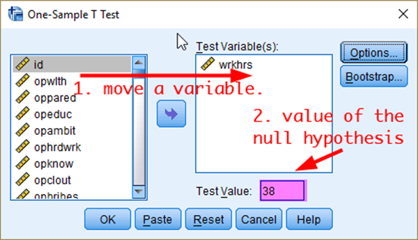
Figure 12: <Figure 12>
Then, 4) click OK. You will see <Figure 13>, which provides the sample mean, the difference from the value that the null hypothesis assumes, t-statistic and its associated p-value. Based on <Figure 13>, do you think Australians work, on average, 38 hours per week? If you are not sure, see the week 9 lecture slides.
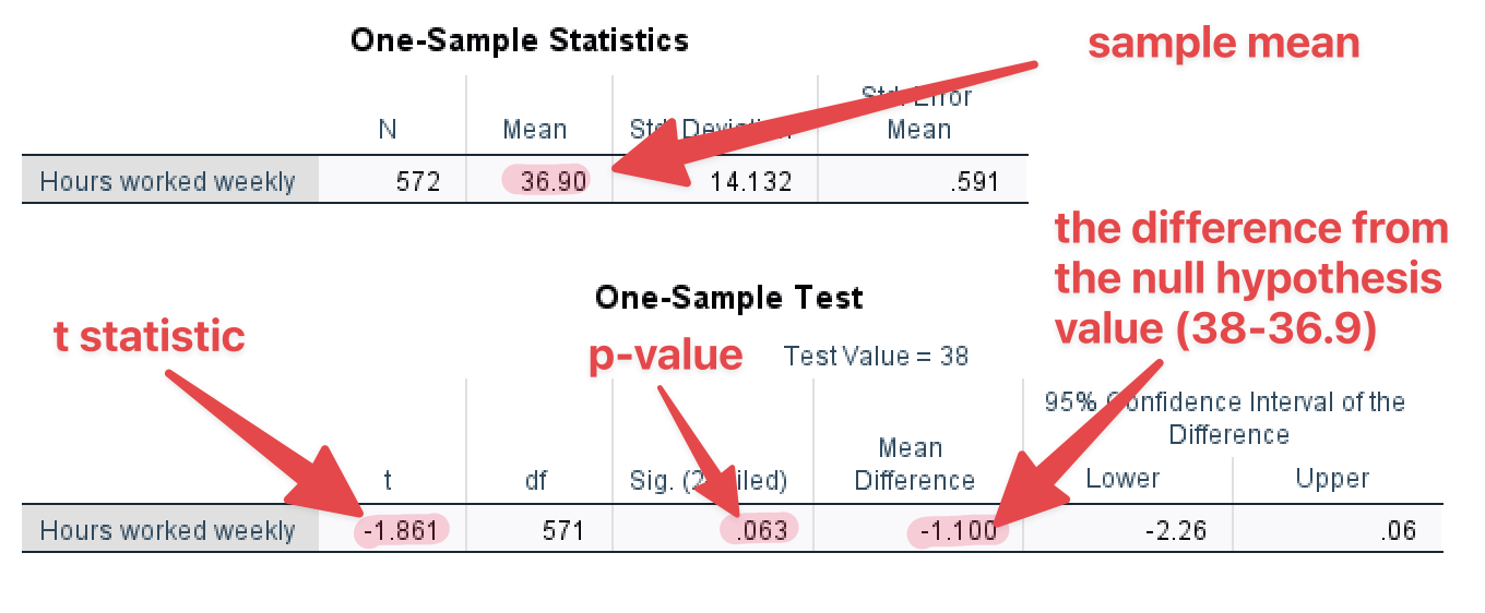
Figure 13: <Figure 13>
NOTE: The p-value in SPSS is based on a two-tailed t-test. If you want to get p-values for a one-tailed t-test, divide the p-value in SPSS by two. For example, if the p-value in SPSS outputs is .025, the p-value for a one-tailed test will be .0125
Two-Sample t-Test
Suppose that we would like to test whether the average working hours are different between men and women. Thus, the null hypothesis is that there is no gender difference in the average working hours. We will use a two-sample t-test because we compare the average working hours between two different groups (men and women).
To conduct two-sample t-test, 1) go to Analyze> Compare Means > Independent-Samples T Test. 2) Move a variable of your interest (in this case wrkhrs) to the box of Test Variable(s) and 3) a variable of Groups (in this case sex) to the box of Grouping Variable. 4) Click Define Groups (see <Figure 14>).
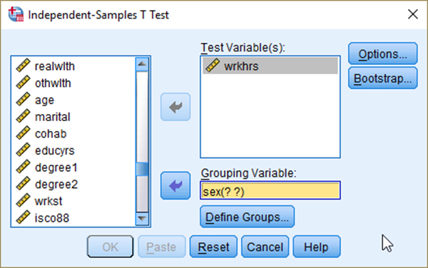
Figure 14: <Figure 14>
In the box of Define Groups, 5) select Use specified values. And 6) input 1 (male) for Group 1 and 2 (female) for Group 2. 7) Click Continue. In the previous box, 8) click OK (see <Figure 15>).
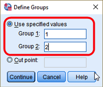
Figure 15: <Figure 15>
Then, you will see <Figure 16>.
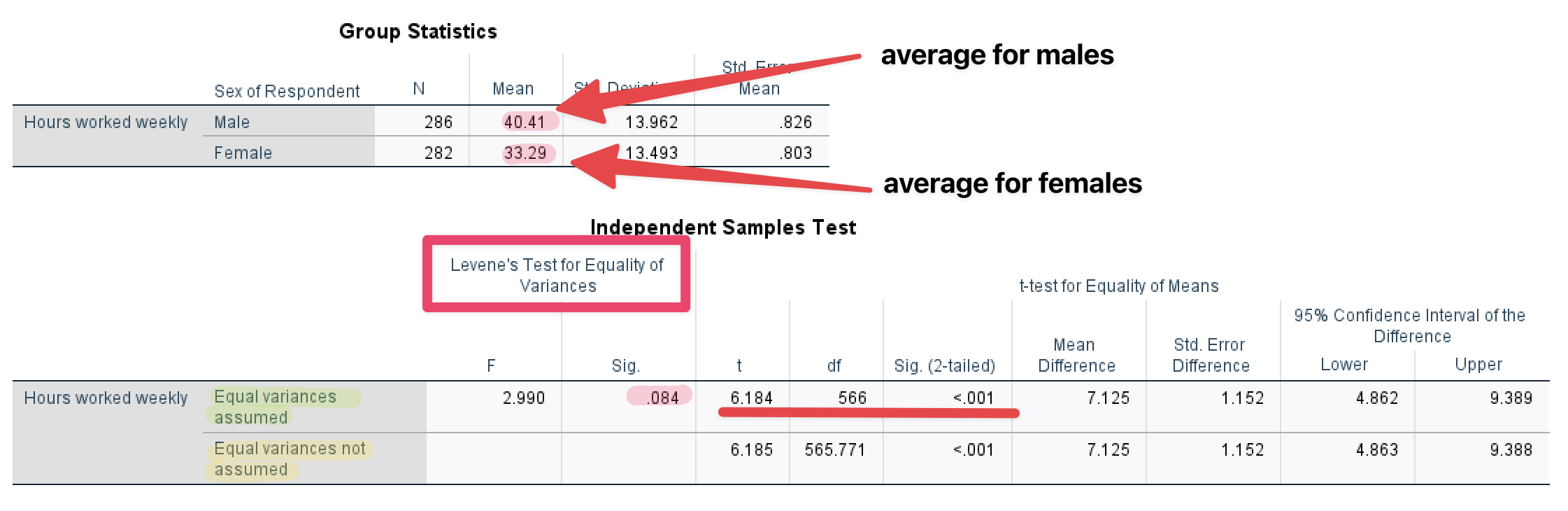
Figure 16: <Figure 16>
Group Statistics in <Figure 16> show the average working hours for males and females, respectively. Independent Samples Test in <Figure 16> examines whether the difference (7.12 = 40.41 – 33.29) is statistically significant.
First, look at the column of “Levene’s Test for Equality of Variance”. This is a test for equal variances. The null hypothesis is that the two distributions (for males and females) have equal variances. Let’s set the significance level .05. <Figure 16> shows that p-value (denoted as Sig.) for Levene’s Test is .084, which is greater than the significance level (.05). Thus, we cannot reject the null hypothesis that the two distributions have the same variance. Therefore, we conclude that the two distributions have equal variances.
For this reason, we will use the t-test for “Equal variances are assumed” (The first row). T statistic is 6.184, and its p-value is less than .001. And this p-value is computed based on two-tailed t-test. Again, let’s set the significance level (α) at .05. The p-value is much less than α, and thus we reject the null hypothesis that there is no gender difference in working hours per week. Therefore, we conclude that there is a significant difference in working hours per week between men and women.
t-Test of Proportion Differences
Suppose that we would like to test whether there is a gender (sex) difference in the proportion of people who think that it is important to come from a wealthy family(newopwlth). Repeat the same procedure as you did in the previous section, but with newopwlth in the box of Test Variable(s) and sex in the box of Grouping Variable (See <Figure 17>).
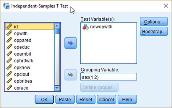
Figure 17: <Figure 17>
Then, you will see <Figure 18>.
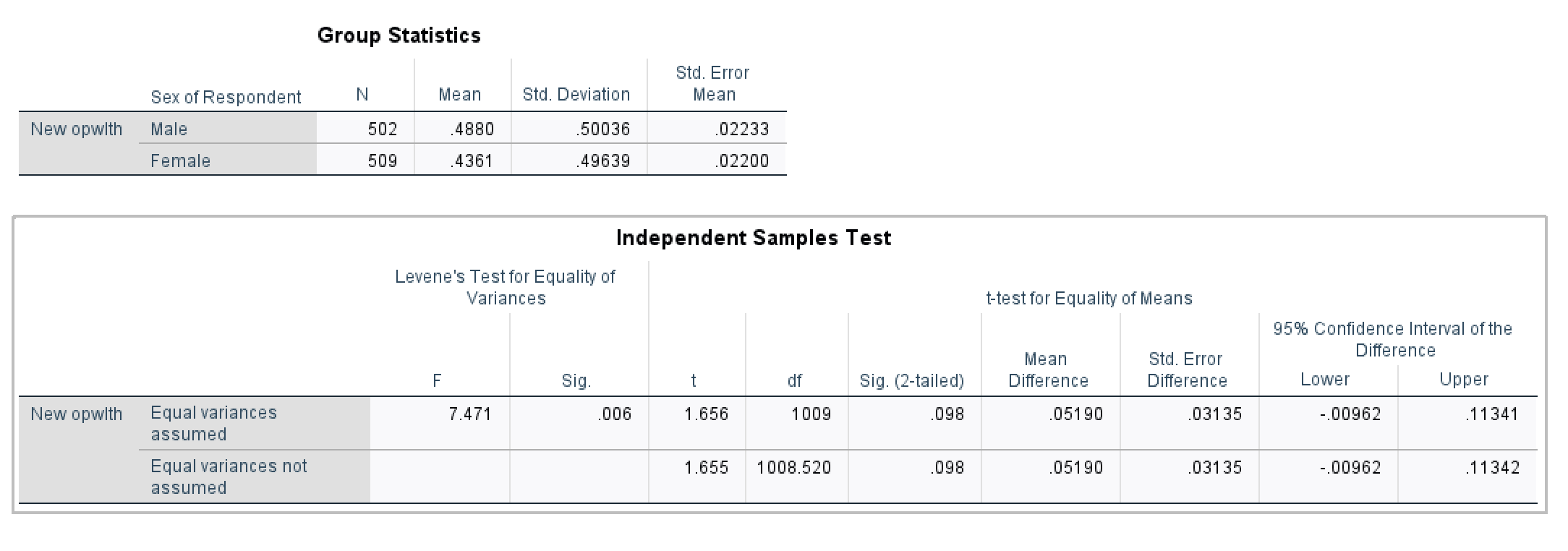
Figure 18: <Figure 18>
Levene’s Test in <Figure 18> shows the p-value is less than the alpha (α=.05). Therefore, the two distributions have a different variance, which enforces you to use “Equal variances not assumed”. The t-statistic is 1.655, and its p-value (.098) is larger than .05. So, we fail to reject the null hypothesis that there is no difference in the proportion of people who think that it is important to come from a wealthy family between men and women at α = .05.Therefore, we conclude that there is no gender difference in assessing the importance of wealthy family background.
Workshop Activity 8: Confidence Intervals and Hypothesis Testing |
||||||||||||||||||||||||
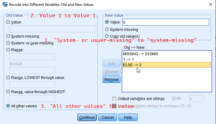
Figure 19: <Figure 19>
|