- Import the 2012 AuSSa dataset.
- How to create a variable of z-scores
- How to compute the z-score of a specific value and its associated probabilities
- How to compute the confidence intervals for continuous variables
- How to compute the confidence interval of proportions
- How to compute confidence intervals for sub-groups
- How to visualise the confidence intervals between groups
- Lab 7 Participation Activity
We will use six packages for this lab. Load them using the following code:
library(dplyr)
library(sjlabelled)
library(sjmisc)
library(summarytools)
library(gmodels)
library(gplots)
Import the 2012 AuSSa dataset.
This lab uses the 2012 AuSSa dataset. You can download the file of this dataset on the course website(iLearn). Download the data file and put it into your working directory. Then, run the following code:
aus2012 <-readRDS("aussa2012.rds")The dataset is loaded as aus2012.
How to create a variable of z-scores
We will make a new variable which is the standardised scores (z-scores) of wrkhrs(hours spent on work per week). std(data name, variable name, append = TRUE) from the sjmisc package will add a variable of standardised scores to your dataset. Run the following code.
aus2012 <- std(aus2012, wrkhrs, append = TRUE)Then, you will see wrkhrs_z added to your dataset. The name of the new variables is always ‘old variable name_z’. Let’s check this newly created variable by running the following code:
aus2012 %>%
  select("id", "wrkhrs", "wrkhrs_z") %>%
  head()
## # A tibble: 6 × 3
## id wrkhrs wrkhrs_z
## <dbl> <dbl> <dbl>
## 1 2.01e15 NA NA
## 2 2.01e15 NA NA
## 3 2.01e15 NA NA
## 4 2.01e15 7 -2.01
## 5 2.01e15 6 -2.08
## 6 2.01e15 NA NAOut of the aus2012 dataset, we select three variables: id, wrkhrs, and wrkhrs_z (If you don’t understand, see Creating a dataset of specific variables. head() shows data for the first six cases. Now you see the original and standardised scores of wrkhrs for the first six cases.
How to compute the z-score of a specific value and its associated probabilities
In the week 8 lecture, you learned how to calculate the z-score of a specific value and find its associated probabilities using the standard normal table. This section will introduce how to perform this job in R.
Suppose that you want to get the z-score of respondents who work 50 hours per week and its associated probabilities. To do this job, you need to run the following code first. Run this code without changing anything.
getZ <- function(v1, v2){
  score <- (v1 -mean(v2, na.rm = TRUE))/sd(v2, na.rm = TRUE)
  prob <- pnorm(abs(round(score, digits = 2)))
  cat(" 1. Z-score for", v1, ":", round(score, digits = 2))
  cat("\n 2. The area between mean and Z-score (B)", ":", round(prob-0.5, digits = 4))
  cat("\n 3. The area beyond Z-score (C)", ":", 0.5-round(prob-0.5, digits = 4))
}
This is a custom code that I made for computing the z-score of a specific value and its associated probabilities. After running this, you will see getZ in the tab of Environment.
Now, compute the z-score of respondents who work 50 hours per week and its associated probabilities using this function. getZ(value, data name$variable name) shows all the necessary information.
getZ(50, aus2012$wrkhrs) ## 1. Z-score for 50 : 0.82
## 2. The area between mean and Z-score (B) : 0.2939
## 3. The area beyond Z-score (C) : 0.2061- First, it shows the z-score.
- Second, it shows the areas between mean and z-score that corresponds to the B areas in the Standard Normal Table that I posted in week 8.
- Third, it shows the areas beyond Z-score that corresponds to the C areas in the Standard Normal Table.
How to compute the confidence intervals for continuous variables
To compute confidence intervals, we use ci() from the gmodels package. ‘ci(data name$variable name, confidence = value, na.rm = TRUE)’ computes the confidence interval of a variable of your choice. For example, you can calculate the confidence interval of wrkhrs using the following code:
ci(aus2012$wrkhrs, confidence = 0.95, na.rm = TRUE)## Estimate CI lower CI upper Std. Error
## 37.5182482 36.5568291 38.4796673 0.4899092In the output, you may see a warning message saying “No class or unkown class. Using default calcuation”. Ignore this warning message. It will not affect your analytic outcome. As long as you see the confidence interval, it is fine. Estimate is the mean. CI Lower is the lower limit of confidence intervals, and CI Upper is the upper limit of confidence intervals. Std. Error is a standard error of a variable. In this output, the average is 37.52, the 95% confidence interval is the range between 36.56 and 38.48, and the standard error is 0.49.
‘na.rm = TURE’ means that cases with missing values are excluded in calculating the confidence intervals. ‘confidence = value’ set the confidence level. In this case, we use 0.95 because we want to get 95% confidence intervals. If you want to get the 90% confidence interval, change the value into 0.90 as in the below code.
ci(aus2012$wrkhrs, confidence = 0.90, na.rm = TRUE)## Estimate CI lower CI upper Std. Error
## 37.5182482 36.7116392 38.3248571 0.4899092How to compute the confidence interval of proportions
The confidence interval of proportions can be computed only for binary variables where values are either 0 or 1. Suppose that we want to calculate the 95% confidence intervals for the proportion of those who agree or strongly agree with the statement that a working mother can establish as warm and secure relationships with her children as a mother who does not work(fechld). First, we need to recode fechld into a binary variable in which 1 = “agree” and 0 = “don’t agree”. Before doing it, please check the labels for fechld in the codebook of the 2012 AuSSa. The below codes recode fechld in such a way (If you don’t understand them, see Recoding variables.
aus2012 <- rec(aus2012, fechld, rec = "1:2=1; 3:5=0", append = TRUE)
aus2012$fechld_r <- set_labels(aus2012$fechld_r,
                               labels = c("agree" = 1, "don't agree" = 0))
Then, run the following code:
ci(aus2012$fechld_r, confidence = 0.95, na.rm = TRUE)## Estimate CI lower CI upper Std. Error
## 0.68343949 0.66040651 0.70647247 0.01174267The output shows the 95% confidence interval of the proportion of people who agree or strongly agree with the statement.
How to compute confidence intervals for sub-groups
We often need to compute the confidence intervals for sub-groups such as male and female respondents. Suppose that we want to calculate the confidence intervals of working hours per week(wrkhrs) for men and women respectively. The first step is to create a dataset for each sub-groups. You learned how to do this in Creating a dataset of a sub-group. The below codes make two datasets, one for male and the other for female respondents.
aus2012.m <- aus2012 %>%
  filter(sex==1)
aus2012.f <- aus2012 %>%
  filter(sex==2)
Then, using these datasets, compute the 90% confidence intervals for men and women. The codes are:
ci(aus2012.m$wrkhrs, confidence = 0.9, na.rm = TRUE) # for male## Estimate CI lower CI upper Std. Error
## 43.7266355 42.6159862 44.8372848 0.6737619ci(aus2012.f$wrkhrs, confidence = 0.9, na.rm = TRUE) # for female## Estimate CI lower CI upper Std. Error
## 32.5876686 31.5609295 33.6144076 0.6230967How to visualise the confidence intervals between groups
Visualising the confidence intervals between groups could be a good way to examine the relationship between variables of groups and your choice. To do this, we use plotmeans() from the gplots package.
‘plotmeans(variable of your choice ~ to_label(group variable), data = data name, p = values for confidence levels, n.label = FALSE, connect = FALSE, xlab = “Label of X-axis”, ylab = “Label of Y-axis”)’ makes the plot of the confidence interval for all groups. The following code generates a plot of 90% confidence intervals for all gender categories.
plotmeans(wrkhrs ~ to_label(sex), data = aus2012, p = 0.90, n.label = FALSE,
          connect = FALSE, xlab = "Gender", ylab = "Hours worked per week")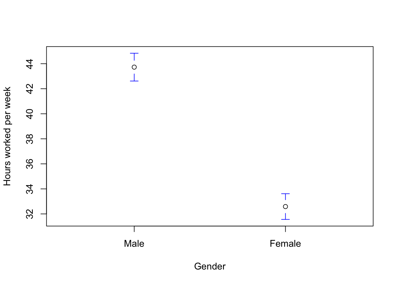
‘n.label = FALSE’ means that the plot does not show the total number of cases for each group. ‘connect = FALSE’ means that the plot does not make lines connected between the average for each group. If you want to draw a connected line, change it into ‘connect = TRUE’.
Note: If the plot is not displayed correctly (e.g., no confidence intervals), increase the size of plot areas. Move your cursor at the border between plot areas and console (see Figure 1). Then, move up while keeping clicking the left mouse button. This will increase the height of plot areas.
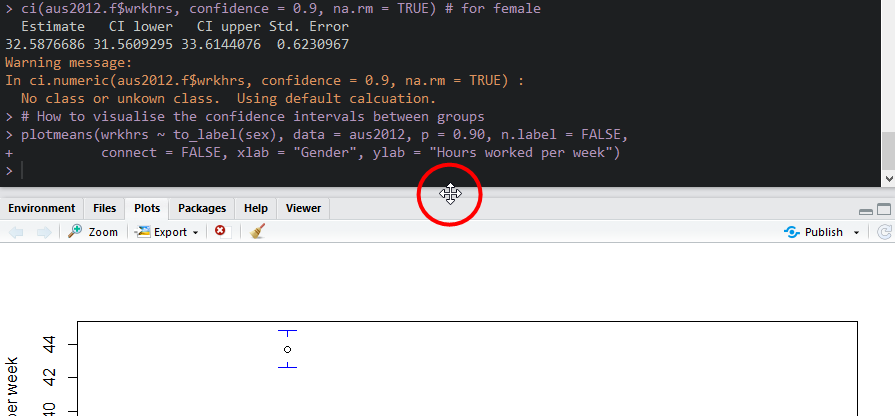
Figure 1: Increase the Size of Plot Areas(1)
Move your cursor at the border between plot areas and right panes (see Figure 2). Then, move right while keeping clicking the left mouse button. This will increase the width of plot areas.
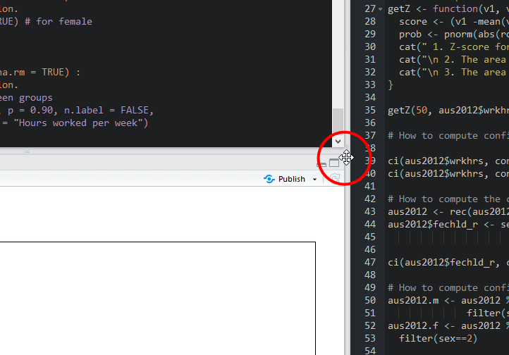
Figure 2: Increase the Size of Plot Areas(2)
After increasing the size of plot areas, run the code for confidence interval plots again. It will show perfect plots.
Lab 7 Participation Activity |
|
No Lab Participation Activity this week. Completing R Analysis Task 2 will contribute to your participation mark. |
The R codes you have written so far look like:
###############################################################################
# Lab 7: Normal Distribution & Confidence Interval
# 3/5/2021
# SOCI8015 & SOCX8015
################################################################################

# Load packages.
library(dplyr)
library(sjlabelled)
library(sjmisc)
library(summarytools)
library(gmodels)
library(gplots)

# Import the 2012 AuSSA dataset
aus2012 <- readRDS("aussa2012.RDS")

# How to create a variable of z-scores
aus2012 <- std(aus2012, wrkhrs, append = TRUE)

aus2012 %>%
  select("id", "wrkhrs", "wrkhrs_z") %>%
  head()

# How to compute the z-score of a specific value and its associated probabilities
getZ <- function(v1, v2){
  score <- (v1 -mean(v2, na.rm = TRUE))/sd(v2, na.rm = TRUE)
  prob <- pnorm(abs(round(score, digits = 2)))
  cat(" 1. Z-score for", v1, ":", round(score, digits = 2))
  cat("\n 2. The area between mean and Z-score (B)", ":", round(prob-0.5, digits = 4))
  cat("\n 3. The area beyond Z-score (C)", ":", 0.5-round(prob-0.5, digits = 4))
}

getZ(50, aus2012$wrkhrs)

# How to compute confidence intervals of numbers
ci(aus2012$wrkhrs, confidence = 0.95, na.rm = TRUE)
ci(aus2012$wrkhrs, confidence = 0.90, na.rm = TRUE)

# How to compute the confidence interval of proportions
aus2012 <- rec(aus2012, fechld, rec = "1:2=1; 3:5=0", append = TRUE)
aus2012$fechld_r <- set_labels(aus2012$fechld_r,
                               labels = c("agree" = 1, "don't agree" = 0))

ci(aus2012$fechld_r, confidence = 0.95, na.rm = TRUE)

# How to compute confidence intervals for sub-groups
aus2012.m <- aus2012 %>%
  filter(sex==1)
aus2012.f <- aus2012 %>%
  filter(sex==2)

ci(aus2012.m$wrkhrs, confidence = 0.9, na.rm = TRUE)
ci(aus2012.f$wrkhrs, confidence = 0.9, na.rm = TRUE)

# How to visualise the confidence intervals between groups
plotmeans(wrkhrs ~ to_label(sex), data = aus2012, p = 0.90, n.label = FALSE,
          connect = FALSE, xlab = "Gender", ylab = "Hours worked per week")