Link to Cheatsheet for manipulating data in dplyr

Note useful functions like:

• filter() - select rows that meet a critiera
• distinct() - remove duplicate rows
• select () - select columns by name
• mutate() - make new variable
• left_join() - joins matching rows on specified column
• bind_rows() - binds rows to bottom of dataset
• bind_cols() - binds columns to right side of dataset
• group_by() - group data into rows with same values - can use to create multiple groups for summary statistics, or regressions

In Figure 1 you can see:

• 2019, SOCI832 Practice.Rproj contains our project information.
• .Rhistory contains the history of the commands we have run.
• .RData holds the data from this project that is currently open, so it can be used if we restart this section.
• nicks_script.R contains the R script we currently have open.

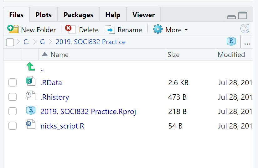
Figure 1: Example of files in the Files Tab.

We run lines of code in this script file by highlighting them and then either:

• pressing Ctrl+Enter (in Windows) or Cmd+Enter (on a Mac) or
• pressing the Run button (below number 12 in Figure 2).

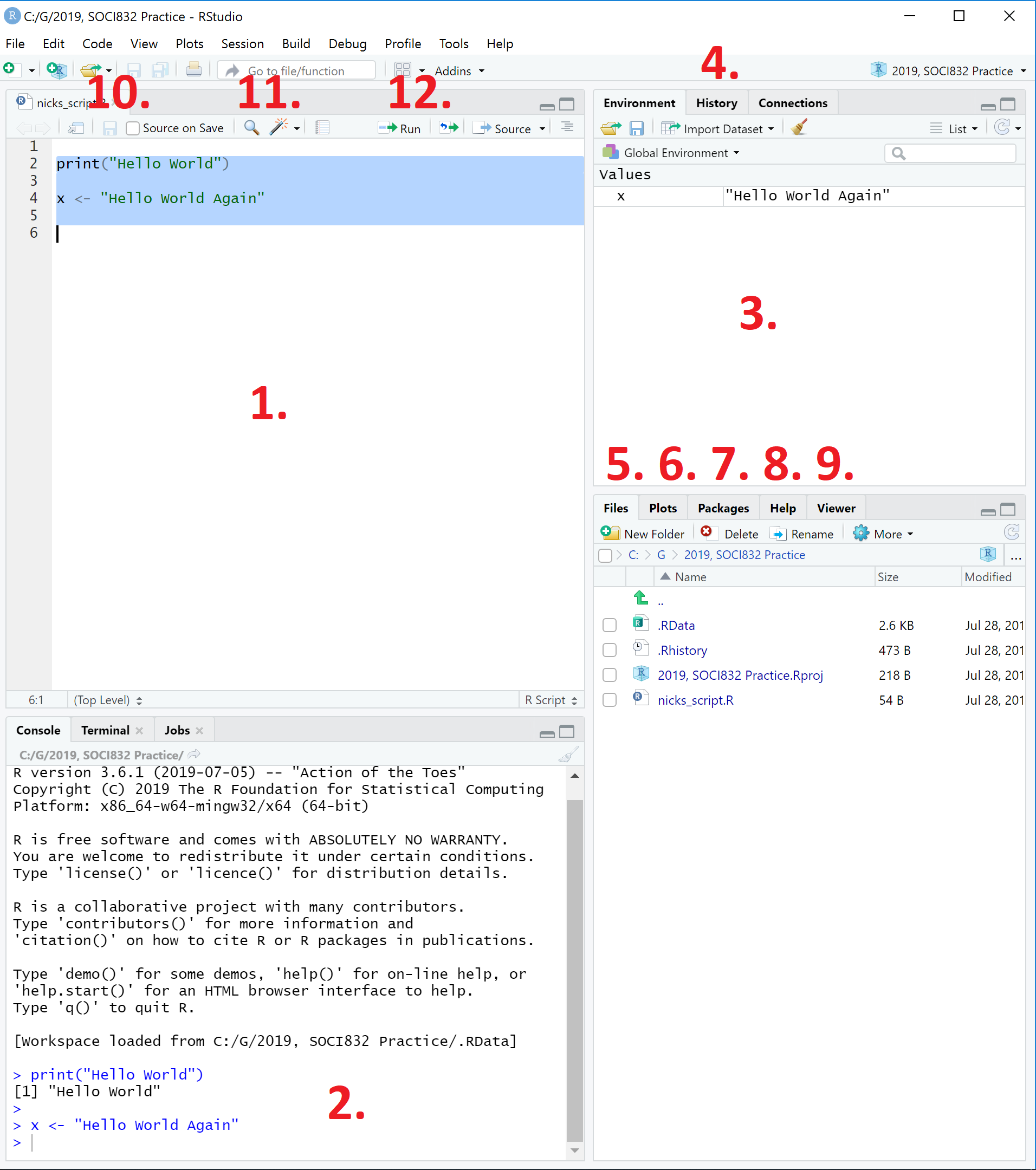
Figure 2: Looking around the RStudio interface.

Tip: Getting help

Google: Often the easiest way to work out how to do something in R is to Google for it. Just type it out as a question ending in “in r”. E.g. how do I delete a variable in r

R helpfiles: These are very good for looking for exact commands and arguments for functions. You can search it by just going to the Help Tab and typing your command in the top right corner. Alternative you can type ?<command name> for an exact search, or ??<command name> for a general search. For example, ?plot will take to you the help screen for the command plot() if it exists, or otherwise will find nothing. If you type ??plot R will search through all R help files and give you a list of files to choose from that contain the word “plot”

One of the most important features of R is the large number of extra functionality that has been written by users across the world. This extra functionality is contained within packages (which is basically synonymous with the word ‘library’).

To run any function from a package, there are two main rules to remember:

1. You need to install the package (using the ‘install.packages()’ command) onto any particular computer ONE TIME ONLY.
2. You need to load the package (using the ‘library()’ command) each time you restart RStudio.

For example, say we wanted to import a dataset that was in excel format. We would need the package ‘readxl’. If we have never used ‘readxl’ before then first we need to install the package.

install.packages("readxl", dependencies = TRUE)

If you run this command in RStudio, you should get a large amount of output that looks something like this:

## Loading required package: readxl

You will know when R has finished running your code, because in the console window the “>” character will appear.

When I ran the command on my own computer, the output was as little different to what is shown above. What output you get will dependent on which other packages you already have installed in R. You might see something like this, with the last few lines of output to the console window being:

## package ‘cellranger’ successfully unpacked and MD5 sums checked
## package ‘Rcpp’ successfully unpacked and MD5 sums checked
## package ‘tibble’ successfully unpacked and MD5 sums checked
## package ‘readxl’ successfully unpacked and MD5 sums checked

## The downloaded binary packages are in
##   C:\Users\nickh\AppData\Local\Temp\RtmpwXzCiK\downloaded_packages
## > |

Before you can run the package, you also need to load the package. To do this you use the ‘library()’ command.

Notice that the library command does not have any inverted commas, while the install packages command does. This is an annoying quirk of R which you need to be aware of.

In most programming languages there is a symbol to tell the program to ignore the rest of the line. In R the comment character is hash: #.

This is useful for

1. putting comments in the code as a note to other users or your future self, and
2. for temporarily turning off a line of code.

As an example of (1) you might write a few lines of code at the top of your R script file:

# Week 1 Code for SOCI832
# by Nicholas Harrigan
# 26/7/2019

As an example of (2), you might put a # in front of the install.packages(“readxl”) command from the previous section and then try to run the whole line.

# install.packages("readxl")

Nothing will happen. You will just return to the “>” character in the console window.

In general I think this is good practice: once you have installed a package, I suggest that you ‘comment out’ the code for that line, so it won’t run again. Installing packages takes time, and you don’t want to do this everytime you run your code

However the code will be there if you ever need to run the code again on a different computer (such as if you give the code to a colleague), or if you reinstall R, when you update R.

Getting your Working Directory: R will always have a directory it looks into first when you ask it to load a dataset or save a file. This is called the ‘Working Directory’.

The advantage of the working directory is that you don’t need to type out the full file path for every file you access.

However, often we aren’t sure what our working directory is, or we want to change it.

If you ever want to know what your working directory is, then you can use the command getwd()

getwd()

## [1] "c:/Users/nickh/methods101/content/docs"

If you want to change your working directory, the command is setwd(). For example:

setwd("C:/G/2019, SOCI832 Practice/")

One thing to note in R is that the slashes between folders aren’t the same as those in Windows.

In R, you can use one of two conventions for separating directories:

1. A single forward slash, i.e. “/” such as

setwd("C:/G/2018, SOCI832/Datasets/AES 2013/")`

2. A double back slash, i.e. “\” such as:

setwd("C:\\G\\2018, SOCI832\\Datasets\\AES 2013\\")

But you cannot use the traditional windows format of a single back slash, i.e. "", such as

> setwd("C:\G\2018, SOCI832\Datasets\AES 2013\")`
Error: '\G' is an unrecognized escape in character string starting ""C:\G"
>

Finding your filepath in Windows: To find your file path right click on the file or folder in Windows Explorer. You should see a menu. Click “Properties”vThe location of the file will be reflected in the “Location” row. You can highlight the whole location and right click to copy it.

When you copy this path back into R, remember to either: (1) add a second forward slash; or (2) change the forward slashes to back slashes. And also remember to include double quotation marks.

Finding your filepath in Mac: Navigate to your file in Finder. Right-click the file. A menu will open up. In the menu, click on “Get Info”. Highlight the text after “Where”. Right click in the highlighted area. In the menu that opens up, click on Copy.

When you copy this path back into R, remember to make sure between the folders there is either: (1) two forward slashes; or (2) one back slash. And also remember to include double quotation marks.

In typesetting there is a distinction between straight quotes (such as ' and ") and curly (or smart) quotes (such as ‘ ’ “ and ”).

R uses straight quotes, such as ' and ".

Microsoft Word uses curly/smart quotes, such as ‘ ’ “ and ”.

If you copy over code that contains quotation marks directly from a website, and the code doesn’t work, delete the copied quotation marks and replace them within RStudio by retyping them.

Microsoft Word’s quotation marks are not compatible with R.

If you are ever looking for how to use RStudio or R, these are a few really helpful ‘cheatsheets’.

• Base R Cheatsheet
• RStudio Cheatsheet

The full list of RStudio Cheatsheets can be found here.

If RStudio hangs and takes a long time. look at the top right of the console window and check if there is a STOP sign displayed in Red. This means that a command is still running. You can press the STOP sign to stop a command.

If you don’t see the STOP sign, or pressing it does nothing, then your other option is to force close RStudio. To do this:

• In Windows: (1) Press simultaneously Ctrl+Alt+Del. (2) Click ‘Task Manager’. (3) In the ‘Processes’ Tab, right click on ‘RStudio’ and select ‘end task’.
• On a Mac: Follow these instructions: https://support.apple.com/en-au/HT201276 Essentially the steps are (1) Press together Option+Command+Esc, and then (2) Select the app in the Force Quit window, then click the Force Quit button.

# Load libraries
library(dplyr)
library(sjPlot)
library(sjmisc)
library(ggplot2)
library(summarytools)



# EXAMPLE 1: NSW CRIME DATASET



# Import dataset
lga <- readRDS(url("https://mqsociology.github.io/learn-r/soci832/nsw-lga-crime.RDS"))

# Calculate the mean unemployment
# because we are going to do two different tables, one for LGAs 
# with unemployment less than mean and one for those with 
# greater than mean.
mean(lga$unemploy, na.rm = TRUE)

# create descriptive statistics table for those lga with
# unemployment less than mean
lga %>% # put the dataset lga into...
  dplyr::group_by(unemploy < 5.68) %>% # creates groups of rows, based on whether they have unempl < or > or =NA
  select(astdomviol,
         astnondomviol, sexoff, robbery, brkentdwel, brkentnondwel) %>% # select these variables
  descr(headings = FALSE,
        stats = c("mean", "sd", "min", "max"), 
        transpose = TRUE) %>%  # produce a descriptive statistics table
  print(method = "browser",
        footnote = NA) # and send it to the browser



# EXAMPLE 2: EUROPEAN UNION DATA (Not provided) DESCRIPTIVES SPLIT BY SEX



#Descriptive statistics - sex - subgroup
euro %>%
  group_by(sex == 1) %>%
  select(v63_r, v64_r, v65_r, v66_r) %>%
  descr(headings = FALSE,
        stats = c("mean", "sd", "min", "max"), 
        transpose = TRUE) %>%
  print(method = "browser",
        footnote = NA)

Removes the words “(Rate per 100,000 population)” from variable labels

library(ggthemes)
library(sjlabelled)
library(sjPlot)

## Install package "strengejacke" from GitHub (`devtools::install_github("strengejacke/strengejacke")`) to load all sj-packages at once!

library(sjmisc)
library(ggplot2)
lga <- readRDS(url("https://mqsociology.github.io/learn-r/soci832/nsw-lga-crime.RDS"))

lga$astdomviol  <- set_label(lga$astdomviol, "Assault - domestic violence")
lga$astnondomviol  <- set_label(lga$astnondomviol, "Assault - non-domestic violence")
lga$sexoff  <- set_label(lga$sexoff, "Sexual Offences")
lga$robbery  <- set_label(lga$robbery, "Robbery")
lga$brkentdwel  <- set_label(lga$brkentdwel, "Break and entering dwelling")
lga$brkentnondwel  <- set_label(lga$brkentnondwel, "Break and entering non-dwelling")
lga$mottheft  <- set_label(lga$mottheft, "Motor vehicle theft")
lga$steafrmot  <- set_label(lga$steafrmot, "Steal from motor vehicle")
lga$steafrsto  <- set_label(lga$steafrsto, "Steal from retail store")
lga$steafrdwel  <- set_label(lga$steafrdwel, "Steal from dwelling")
lga$steafrprsn  <- set_label(lga$steafrprsn, "Steal from person")
lga$fraud  <- set_label(lga$fraud, "Fraud")
lga$damtoprpty  <- set_label(lga$damtoprpty, "Malicious damage to property")
lga$hrssthreat  <- set_label(lga$hrssthreat, "Harassment and threatening")
lga$recvstlgoods  <- set_label(lga$recvstlgoods, "Receiving stolen goods")
lga$oththeft  <- set_label(lga$oththeft, "Other theft")
lga$arson  <- set_label(lga$arson, "Arson")
lga$marijuana  <- set_label(lga$marijuana, "Possession use of cannabis")
lga$weapon  <- set_label(lga$weapon, "Prohibited weapons offences")
lga$trespass  <- set_label(lga$trespass, "Trespass")
lga$offcond  <- set_label(lga$offcond, "Offensive conduct")
lga$offlang  <- set_label(lga$offlang, "Offensive language")
lga$liqoff  <- set_label(lga$liqoff, "Liquor Offences")
lga$brchavo  <- set_label(lga$brchavo, "Breach AVO")
lga$brchbailcon  <- set_label(lga$brchbailcon, "Breach bail condition")
lga$rsthindofficer <- set_label(lga$rsthindofficer,"Resist or hinder officer")
lga$transport <- set_label(lga$transport, "Transport regulatory offences")