The second lab session covers the following:
- How to enter data manually
- How to save R files
- How to install packages in RStudio
The goal of this lab is to make you familiarised with dataframes. You will enter the data of four variables collecting from 30 respondents.
How to enter data manually
It is not often the case that researchers have to construct datasets by themselves. They often use secondary datasets which were generated and released by others. Sometimes they hire survey companies for collecting and creating datasets. In this lab you are required to construct a small dataset by yourself because I believe this is the best way to understand the structure of datasets (or data frames).
We will enter manually a subsample of 30 respondents from Aussa (Australian Survey of Social Attitudes) dataset using Table 1. It shows the information on four variables: gender, age, political orientation and social class.
The questionnaires used for this dataset are:
(1) Male
(2) Female
(999) Don’t know; No answer; refused
2. How old are you?
(________) years old
(999) Don’t know; No answer; Refused
3. In politics, people often talk about left or right. Where would you put yourself among the following?
(1) Far left
(2) Left
(3) Center
(4) Right
(5) Far right
(999) Don’t know; No answer; Refused
4. Most people see themselves as belonging to a particular class. Please tell me which social class you would say you belong to?
(1) Lower class
(2) Working class
(3) Lower middle class
(4) Middle class
(5) Upper middle class
(6) Upper class
(999) Don’t know; No answer; Refused
Table 1 shows the responses to those four questions from 30 respondents.
| Gender | Age | Political Orientation | Social Class |
|---|---|---|---|
| Male | 66 | Right | Middle class |
| Female | 72 | Right | Upper middle class |
| Female | 59 | Left | Middle class |
| Female | 20 | Left | Lower middle class |
| Female | 68 | Right | Upper middle class |
| Male | 76 | Right | Middle class |
| Male | 61 | Left | Upper middle class |
| Male | 90 | Right | Middle class |
| Female | 64 | Left | Lower middle class |
| Female | 39 | Left | Upper middle class |
| Male | 57 | Right | Middle class |
| Male | 47 | Left | Lower class |
| Female | 56 | Left | Middle class |
| Female | 51 | Left | Middle class |
| Male | 34 | Left | Working class |
| Male | 18 | Center | Middle class |
| Female | 18 | Left | Working class |
| Female | 30 | Left | Upper middle class |
| Female | 65 | Right | Middle class |
| Male | 35 | Right | Middle class |
| Female | 44 | Right | Upper class |
| Female | 40 | Right | Middle class |
| Male | 57 | Left | Upper middle class |
| Male | 40 | Left | Lower middle class |
| Female | 59 | Left | Middle class |
| Female | 82 | Right | Middle class |
| Female | 44 | Far right | Working class |
| Female | 30 | Left | Middle class |
| Male | 77 | Left | Working class |
| Female | 60 | Right | Lower middle class |
Step 1: Creating a CSV file using Excel
It is possible to enter data in R. However, I don’t recommend this entering method because it is not an easy and efficient way of making datasets. Instead, we will use Excel (or any spreadsheet program) for entering data, and then import the file of Excel-format data into R.
Open Excel and look at Table 1. When you enter gender information, you may start by entering either “Male” or “Female”. However, typing texts is not an efficient way of entering data. Instead, we will enter numbers which will be linked to each gender category. Look at the questionnaire 1. You will see 1 is assigned for males and 2 is for females. Thus, we will enter 1 for males and 2 for females. For the same reason, we will use numbers instead of texts in entering data of the other three variables. In addition, we will make a new variable, identification numbers (id), which is a unique number assigned to each respondent. The identification number for the first respondent is 1, that for the second is 2, and finally, that for the 30th is 30. Also, we need to make a variable name in a simple way. Most important is that the variable name should have no space in it. Otherwise, it would be more likely that R can’t recognize variable names.
I assign variable names as in the below.
- id: identification number
- sex: gender
- age: age
- polorient: political orientation
- class: social class
Your final dataframe will look like Table 2.
| id | sex | age | polorient | class |
|---|---|---|---|---|
| 1 | 1 | 66 | 4 | 4 |
| 2 | 2 | 72 | 4 | 5 |
| 3 | 2 | 59 | 2 | 4 |
| 4 | 2 | 20 | 2 | 3 |
| 5 | 2 | 68 | 4 | 5 |
| 6 | 1 | 76 | 4 | 4 |
| 7 | 1 | 61 | 2 | 5 |
| 8 | 1 | 90 | 4 | 4 |
| 9 | 2 | 64 | 2 | 3 |
| 10 | 2 | 39 | 2 | 5 |
| 11 | 1 | 57 | 4 | 4 |
| 12 | 1 | 47 | 2 | 1 |
| 13 | 2 | 56 | 2 | 4 |
| 14 | 2 | 51 | 2 | 4 |
| 15 | 1 | 34 | 2 | 2 |
| 16 | 1 | 18 | 3 | 4 |
| 17 | 2 | 18 | 2 | 2 |
| 18 | 2 | 30 | 2 | 5 |
| 19 | 2 | 65 | 4 | 4 |
| 20 | 1 | 35 | 4 | 4 |
| 21 | 2 | 44 | 4 | 6 |
| 22 | 2 | 40 | 4 | 4 |
| 23 | 1 | 57 | 2 | 5 |
| 24 | 1 | 40 | 2 | 3 |
| 25 | 2 | 59 | 2 | 4 |
| 26 | 2 | 82 | 4 | 4 |
| 27 | 2 | 44 | 5 | 2 |
| 28 | 2 | 30 | 2 | 4 |
| 29 | 1 | 77 | 2 | 2 |
| 30 | 2 | 60 | 4 | 3 |
Start entering Table 2 in Excel. Variable names should be entered in the first row (See Figure 1).
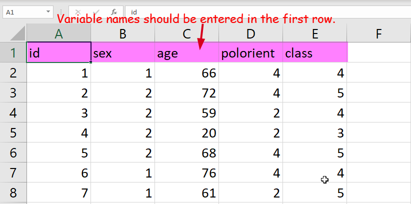
Figure 1: Entering Data in Excel
Once you complete entering the data, save your data as a format of CSV (Comma delimited) (for Windows; See Figure 2) or CSV UTF-8 (Comma-delimited) (.csv) (for Mac; See Figure 3) in your R WORKING DIRECTORY (). Otherwise, you can’t import this file into R. I set “table-1-30-respondents” as the file name (See Figure 2 and 3). Click Save.
Note: If you are not sure about what R working directory is, see “Setting your default working directory” in Lab 1.
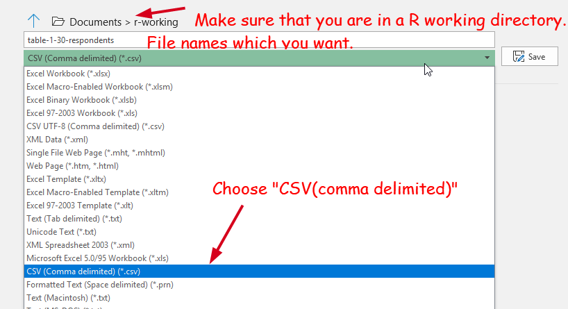
Figure 2: Saving as CSV Files for Windows
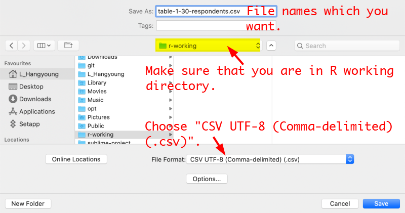
Figure 3: Saving as CSV Files for Mac
Step 2: Importing CSV Files
Open RStudio. You will see the tab of “Untitled1” in the “Source” window. We will expand the “Source” window so that we can have more spaces to write R codes. Click the square icon in the “Source” window (See Figure 4). The “Source” window will be expanded vertically.
Figure 4: Expanding Source Pane
In this “Source” window, we will write R codes. First, write the following codes (See Figure 4).
mydata <- read.csv("table-1-30-respondents.csv")This is the code for importing CSV files into R.
- mydata is a data name I assign. You can assign any name as you want.
- <- has the same meaning as equal sign(=).
- read.csv(“file name”) is the code for importing CSV files. You need to specify your file name between double quotation marks.
Overall, the meaning of this code is: 1) import the “table-1-30-respondents.csv” files from your working directory. 2) the name of the imported data is mydata.
Next, we need to execute this code. Move the mouse cursor at the line you want to execute. Then, hit Ctrl+Enter (For Mac, hit Cmd+Enter). Make sure that you have to hit the two keys simultaneously. Then, You will see that your code is transferred and executed in the “Console” window. After executing the line of code, RStudio automatically advances the cursor to the next line. This enables you to single-step through a sequence of lines (See Figure 5).
Note: If you fail to import CSV files, please check the warning message in your R console. In case you see “No such file or directory” in the warning message, it tells you that R cannot find your CSV files. Check whether your CSV files are in your working directory and the file name is correctly specified (Note that R distinguishes uppercase and lowercase letters, and thus the file name should be exactly the same).
Step 3: Check Imported Datasets
Let’s check whether the dataset is imported correctly.
mydata## id sex age polorient class
## 1 1 1 66 4 4
## 2 2 2 72 4 5
## 3 3 2 59 2 4
## 4 4 2 20 2 3
## 5 5 2 68 4 5
## 6 6 1 76 4 4
## 7 7 1 61 2 5
## 8 8 1 90 4 4
## 9 9 2 64 2 3
## 10 10 2 39 2 5
## 11 11 1 57 4 4
## 12 12 1 47 2 1
## 13 13 2 56 2 4
## 14 14 2 51 2 4
## 15 15 1 34 2 2
## 16 16 1 18 3 4
## 17 17 2 18 2 2
## 18 18 2 30 2 5
## 19 19 2 65 4 4
## 20 20 1 35 4 4
## 21 21 2 44 4 6
## 22 22 2 40 4 4
## 23 23 1 57 2 5
## 24 24 1 40 2 3
## 25 25 2 59 2 4
## 26 26 2 82 4 4
## 27 27 2 44 5 2
## 28 28 2 30 2 4
## 29 29 1 77 2 2
## 30 30 2 60 4 3mydata is the name of data I assigned. If you write and execute the data name, R will show the data frame (See Figure 5).
Figure 5: Writing and Running Codes in RStudio
Another way to see the data frame is to click the data name in the tab of Environment tab. Environment tab shows all datasets that you import into R. Click the name of data you want to see. This will show the data frame. You can close the data frame by clicking the icon of x (See Figure 6)
Figure 6: How to See Data Frames
Step 4: Saving Your R Codes
Let’s save our R codes you have written so far so that you can import and work on it again next time. Click the icon of disks in the top menu of the “Source” window (See Figure 7).
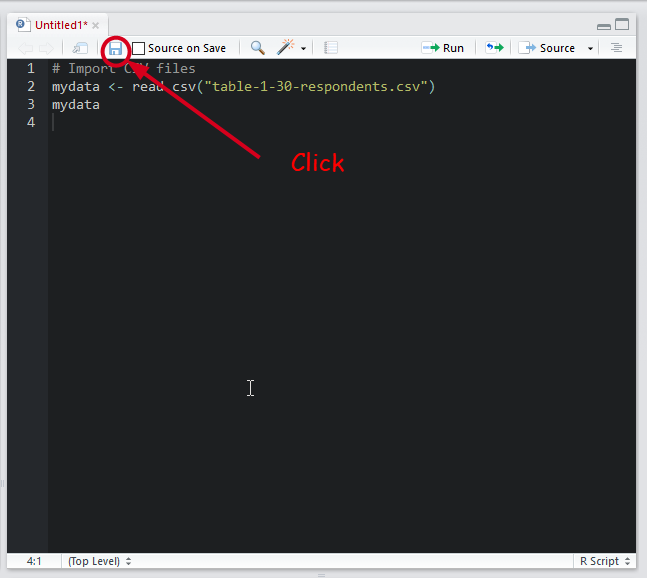
Figure 7: Saving R Files
In a newly popped-up window, type “myRcode-1.R” in the “File name”. Note that the file name should end with “.R”, which means the file type is an R code file. Then, click on “Save” (See Figure 8 for Windows or Figure 9 for Mac). This will save your R file in your working directory. Also, you will see the tab of “Untitled” changed into “myRcode-1.R”.
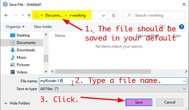
Figure 8: Saving R Files for Windows
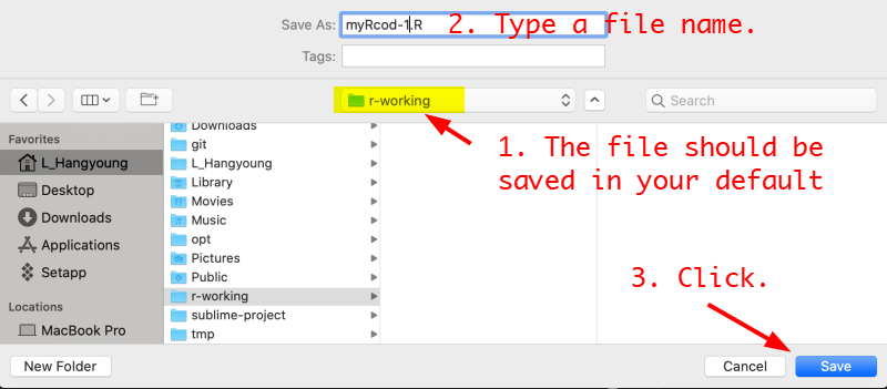
Figure 9: Saving R Files for Mac
Close RStudio (Do not save workspace image when it is asked) and open it again. If you followed all my instructions in Lab 1, you will see the file of “myRcode-1.R” is automatically loaded. If not, review “Automatically loading your previous R codes” in Lab 1.
In the next lab, we will keep working on this 30 respondent dataset and the R file we have made so far. Thus, please keep all the files.
But I am asking you to do one final thing before closing the lab 2. We will install several R packages that will be used throughout the remaining labs.
How to install packages in RStudio
R packages are a collection of R functions, sample datasets, and compiled codes developed by the R developer community. Base R (which you installed in Lab 1) provides just essential functions. To conduct more complicated analyses, it would be easier and more efficient to take advantage of predefined R functions that are widely used by researchers. Installing packages is an easy way to access and use such popular R functions. Currently, there are more than 10,000 R packages which are available for free. Out of them, we will use seven packages throughout the course. They are:
- gmodels
- gplots
- sjlabelled
- sjmisc
- sjPlot
- summarytools
- tidyverse
Let’s start installing these packages. First, we will install gmodels package (See Figure 10).
- Open RStudio.
- Click on the Packages tab in the bottom left pane and then click on install. This will open a new window.
- Type the name of packages you want to install (in this case gmodels) in the section of Packages. You can install multiple packages at one time, but each package name should be separated with space or comma (e.g., “gmodels, gplots, sjlabelled”) Also, make sure that the box of “Install dependencies” should be ticked, which enables R to install other packages that are required for running the package of your choice.
- Click on OK. RStudio will start installing packages.
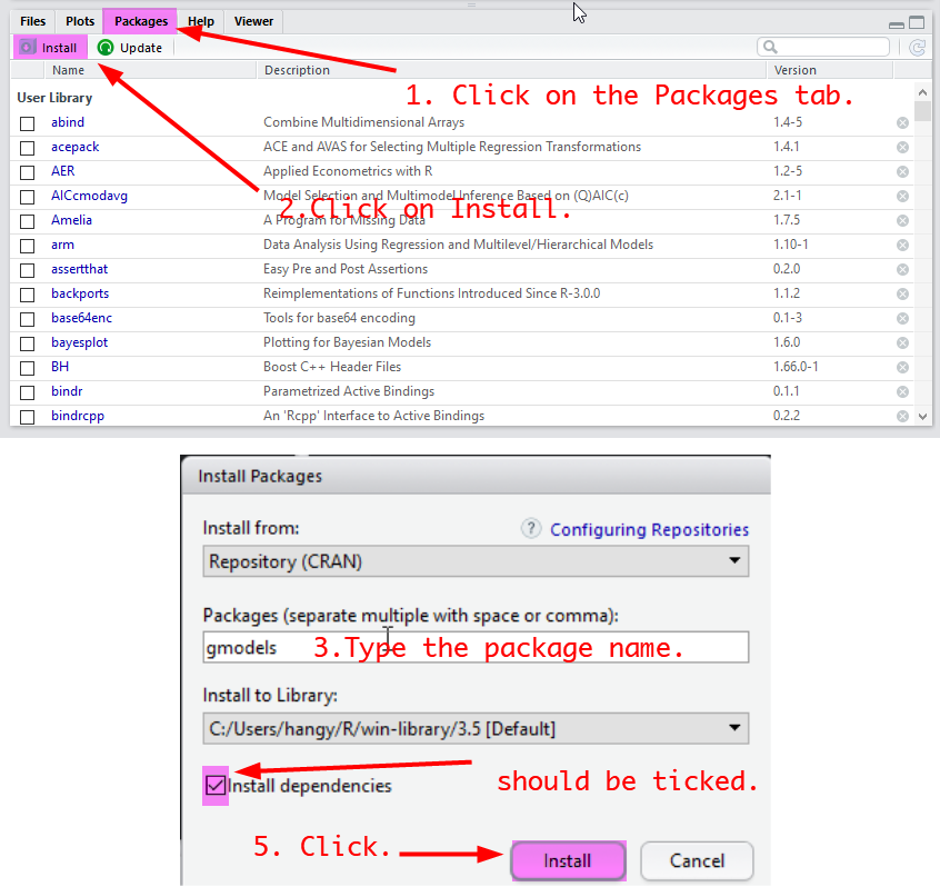
Figure 10: Installing Packages
Note: It is recommended to update installed R packages. An easy way to update them is to click on Update in the Package tab.
Alternatively, you can also install packages using an R code. In the R Console, type the following code:
install.packages("gmodels", dependencies = TRUE)Then, hit Enter (for Windows) or Return (for MacOS). It will start installing the gmodels packages. Package names should be enclosed by double quotation marks. Otherwise, R cannot recognise the package name and will show an error message.
Note: Installed packages can be updated by an R code. For example, if you want to update the gmodels package. execute the following code in your R Console:
update.packages("gmodels")
Lab 2 Participation Activity |
Note: Please complete the Lab 2 Participation Activity. You can find the link to this activity on iLearn. This activity will contribute to your participation marks. |