The third lab session covers the following:
- How to replicate labs easily
- How to make variables
- How to assign variable labels
- How to assign value labels
- How to save datasets
Easy way to replicate labs
In every lab, you are required to run many R codes, which means that you should type lots of codes. In typing codes, it is common to make mistakes. You can miswrite codes, which will show error messages in the Console when you execute them.
To avoid this kind of inconvenience and trouble, I would like to introduce an easy way to replicate lab R codes and outcomes. Follow the below steps (See Figure 1).
Open RStudio and open a new R Script. If you are not sure how to do this, see Figure 3 in Lab1.
Go to https://methods101.com.au. Click the lab you want to study. At the bottom of each lab, you can find all the codes used in the lab. Select and copy all the R codes.
Paste the selected R codes in a newly opened R script.
Save the R script in your working folder. If you are not sure how to do this, see Saving Your R Codes.
Then, you can run the codes without typing them all.
Note: When you look at R codes at the bottom, you may notice that the first line starts with a hashtag(#). Any line beginning with a hashtag(#) is a comment for codes in which researchers often put explanations about codes. When you write new codes with which you are not familiar, it would always be useful to add comments for them. Otherwise, you may forget the meaning of those codes when you work with them again in the future.
Figure 1: Easy Way to Replicate R Codes
Import the dataset that you constructed in Lab 2
We continue working on the dataset we created in the last lab. Open RStudio, and you will see the R file you made in the last lab. If you do not see your R file, go to File >> Open File… in the top menu. And open it from your working directory. Then, run all the codes you wrote in the previous lab.
The code you shoud run is:
mydata <- read.csv("table-1-30-respondents.csv")You will see mydata in the tab of Environment.
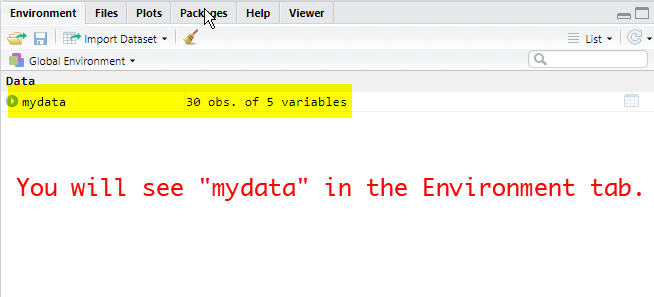
Figure 2: Check Your Data
Now, you are ready to learn new codes.
Playing with variables
R is a calculator.
Just think of R as a calculator. It can compute elementary equations. Examples are:
250 + 125## [1] 375250 - 125## [1] 125250 * 125## [1] 31250250/125## [1] 2As expected, R can do complicated equations as well. The example below computes \({e}^{5}+\sqrt{\frac{\ln{253}+\pi}{653-258}}\).
exp(5)+sqrt((log(253) + pi)/(653-258))## [1] 148.5614If you want to learn more about basic mathematical operations in R, go to Basic Operations in R Tutorial.
How to make variables
In R, variables can take several forms. In this lab, we will cover 1) numbers, 2) characters, and 3) data frames that are essential for the course. If you want to study more about variables in R, see Variable Types in R Tutorial.
A variable could be a single number. For instance, we can assign 5 to variable a.
a <- 5The <- tells R to assign a number to the name of variables in the right (in this case, a). If you want to see numbers assigned to variables, type the variable name and run it. It will show the numbers.
a## [1] 5R can assign the outcomes of mathematical operations to variables. For example,
b <- a * a + 3
b
## [1] 28Now, we have two variables (a and b). Let’s use them. Can you guess what the outcome will be if we add a and b? Let’s check the result.
a + b## [1] 33In addition, R can assign texts to variables. In R, this form of data is called characters; any value written within a pair of single or double quotes in R is treated as a character. For example,
c <- "soci 8015"
c
## [1] "soci 8015"Note that you can also make a list of values (called a vector in R) and assign it to a variable. For example, we are going to input age and gender for five respondents.
age <- c(36, 19, 30, 55, 42)
age
## [1] 36 19 30 55 42gender <- c("male", "female", "female", "male", "female")
gender## [1] "male" "female" "female" "male" "female"age is a list of numbers, and gender is a list of characters. If you want to confirm this, run the following code:
class(age)## [1] "numeric"class(gender)## [1] "character"Now, we will make a data frame by combining age and gender that we just created.
data <- cbind(age, gender)
data <- as.data.frame(data)Let’s check the data frame we just made and also the type of variable.
data## age gender
## 1 36 male
## 2 19 female
## 3 30 female
## 4 55 male
## 5 42 femaleclass(data)## [1] "data.frame"How to remove variables we made so far.
So far, we have made seven variables: mydata, a, b, c, age, gender, and data. However, we will keep only mydata which will be used in the remaining lab.
If you want to remove only one variable, use ‘rm(variable name)’. For example,
rm(a)If you want to remove multiple variables, use ‘rm(variable name 1, variable name 2, variable name 3, ...)’. For example,
rm(b, c, age, gender, data)Check the tab of Environment. You will see the variables you listed are removed.
Assigning labels and value labels to the AuSSa subsample dataset
The remaining lab will work on the AuSSA subsample dataset you created in Lab 2. We will assign labels and value labels to each variable.
Loading packages
For labelling data, we need to use two packages which I recommended to install in the lab 2: sjlabelled and sjmisc. To load them in R, run the following codes:
library(sjlabelled)
library(sjmisc) Every time you want to use packages, you need to run library(package name). Otherwise, you will see a warning message that says “could not find function”.
How to access variables in a data frame.
A data frame consists of many variables. For instance, mydata consists of five variables: id, sex, age, polorient, class. We learned how to see a data frame (typing data names and running them will show data frames). But we do not know how to see a specific variable in a data frame. To access it, use data frame name$variable name. For example, the following codes will show each of four variables in mydata.
mydata$sex## [1] 1 2 2 2 2 1 1 1 2 2 1 1 2 2 1 1 2 2 2 1 2 2 1 1 2 2 2 2 1 2mydata$age ## [1] 66 72 59 20 68 76 61 90 64 39 57 47 56 51 34 18 18 30 65 35 44 40 57 40 59
## [26] 82 44 30 77 60mydata$polorient## [1] 4 4 2 2 4 4 2 4 2 2 4 2 2 2 2 3 2 2 4 4 4 4 2 2 2 4 5 2 2 4mydata$class## [1] 4 5 4 3 5 4 5 4 3 5 4 1 4 4 2 4 2 5 4 4 6 4 5 3 4 4 2 4 2 3How to add variable labels
It is recommended to add short descriptions of variables which I call ‘variable labels’. We often set variable names in a simple way such as polorient. Consequently, it is easy to forget what variables are about after a while. In that case, variable labels will be helpful for recalling them.
First, check the variable label of id. get_label(data name$variable name) will show a variable label.
get_label(mydata$id)## NULLExpectedly, it shows nothing (= NULL). So, we need to assign the variable label for id.
mydata$id <- set_label(mydata$id, label = "Identification Number")
get_label(mydata$id)## [1] "Identification Number"data name$variable name <- set_label(data name$variable name, label = "variable label") will assign “variable labels” to specified variables. After assigning it, get_label function will show the newly assigned variable label.
Let’s assign variable labels to the other variables as well.
mydata$sex <- set_label(mydata$sex, label = "Gender")
mydata$age <- set_label(mydata$age, label = "Age")
mydata$polorient <- set_label(mydata$polorient, label = "Political Orientation")
mydata$class <- set_label(mydata$class, label = "Social Class")How to add value labels
When we constructed the dataset in lab 2, we entered numbers instead of texts. Nonetheless, the number itself has no meaning except for age. Therefore, it is recommended to assign a (category) label to each value (number). Category information of each variable can be found in Lab 2: How to enter data manually. For example, in sex “Male” will be assigned to 1, and “Female” will be assigned to 2. We will use set_labels function for this purpose. The R code is data name$variable name <- set_labels(data name$variable name, labels = c("category 1" = value 1, "category 2" = value 2, ...)).
mydata$sex <- set_labels(mydata$sex, labels = c("male" = 1, "female" = 2))Note
When you run the above code to assign value lables to sex variable, you might see a warning message saying:
“Error in set_labels_helper(x = .dat, labels = labels, force.labels = force.labels, :
Package `haven’ required for this function. Please install it.”
To fix this problem, run the following code.
install.packages("haven")The code will install ‘haven’ package.
Instead, you can install it following the way you learned in Lab 2.
Then, let’s assign value labels to polorient and class as well.
mydata$polorient <- set_labels(mydata$polorient,
labels = c("Far left" = 1,
"Left" = 2,
"Center" = 3,
"Right" = 4,
"Far right" = 5))
mydata$class <- set_labels(mydata$class, labels = c("Lower class" = 1,
"Working class" = 2,
"Lower middle class" = 3,
"Middle class" = 4,
"Upper middle class" = 5,
"Upper class" = 6))Now is the time to check whether you followed all the steps so far correctly. We will make frequency tables of sex, polorient and class using frq function (you will learn more about this function in lab 5). If you followed well, you will see the variable and value labels of the tree variables.
frq(mydata$sex)##
## Gender (x) <integer>
## # total N=30 valid N=30 mean=1.60 sd=0.50
##
## Value | Label | N | Raw % | Valid % | Cum. %
## ----------------------------------------------
## 1 | male | 12 | 40 | 40 | 40
## 2 | female | 18 | 60 | 60 | 100
## <NA> | <NA> | 0 | 0 | <NA> | <NA>frq(mydata$polorient)##
## Political Orientation (x) <integer>
## # total N=30 valid N=30 mean=2.93 sd=1.05
##
## Value | Label | N | Raw % | Valid % | Cum. %
## -------------------------------------------------
## 1 | Far left | 0 | 0.00 | 0.00 | 0.00
## 2 | Left | 16 | 53.33 | 53.33 | 53.33
## 3 | Center | 1 | 3.33 | 3.33 | 56.67
## 4 | Right | 12 | 40.00 | 40.00 | 96.67
## 5 | Far right | 1 | 3.33 | 3.33 | 100.00
## <NA> | <NA> | 0 | 0.00 | <NA> | <NA>frq(mydata$class)##
## Social Class (x) <integer>
## # total N=30 valid N=30 mean=3.77 sd=1.14
##
## Value | Label | N | Raw % | Valid % | Cum. %
## ----------------------------------------------------------
## 1 | Lower class | 1 | 3.33 | 3.33 | 3.33
## 2 | Working class | 4 | 13.33 | 13.33 | 16.67
## 3 | Lower middle class | 4 | 13.33 | 13.33 | 30.00
## 4 | Middle class | 14 | 46.67 | 46.67 | 76.67
## 5 | Upper middle class | 6 | 20.00 | 20.00 | 96.67
## 6 | Upper class | 1 | 3.33 | 3.33 | 100.00
## <NA> | <NA> | 0 | 0.00 | <NA> | <NA>If you followed all the stpes correctly, the frequency table will show variable and value labels
Saving data into RDS format
Now, you have a dataset with full information. So, you need to save it for your future use. There are multiple ways to save datasets in R. However, I recommend to save them in RDS format because this format preserves data structure and reduces the size of files considerably. The R code for this job is saveRDS(data name, file = "file-name.rds"). Note that the file name should end with “.rds”.
saveRDS(mydata, file = "mydata.rds")After running this code, go to your working directory. You will see “mydata.rds” there. Also, do not forget to save your R file again. If you click on the icon of disk in the text editor, your R file will be saved.
The next lab will introduce how to import RDS file into R. So, please keep “mydata.rds”.
Lab 3 Participation Activity |
|
If you follow all the instructions correctly, you will find “mydata.rds” in your working directory. “mydata.rds” is the data file you have been working on so far. Please send “mydata.rds” in your wokring directory to the unit convenor (hangyoung.lee@mq.edu.au) by email. The unit convenor will check whether your data file is created correctly. This activity will contribute to your participation marks.If you have any issues in generating “mydata.rds”, do not hesitate to contact the unit convenor. |
The R codes you have written so far look like:
################################################################################
# Title: Lab 2 & 3
# Course: SOCI8015 & SOCX8015
# Date: 14/03/2022
################################################################################
# Import CSV files
mydata <- read.csv("table-1-30-respondents.csv")
mydata
# Elementary equations
250 + 125
250 - 125
250 * 125
250/125
# A complicated equation
exp(5)+sqrt((log(253) + pi)/(653-258))
# Make variables
a <- 5
a
b <- a * a + 3
b
a + b
c <- "soci 8015"
c
# Create vectors
age <- c(36, 19, 30, 55, 42)
age
gender <- c("male", "female", "female", "male", "female")
gender
class(age)
class(gender)
# Create data frames
data <- cbind(age, gender)
data <- as.data.frame(data)
data
class(data)
# How to remove variables
rm(a)
rm(b, c, age, gender, data)
# Load package
library(sjlabelled)
library(sjmisc)
# How to access variables in data frame
mydata$sex
mydata$age
mydata$polorient
mydata$class
# How to add variable labels
get_label(mydata$id)
mydata$id <- set_label(mydata$id, label = "Identification Number")
get_label(mydata$id)
mydata$sex <- set_label(mydata$sex, label = "Gender")
mydata$age <- set_label(mydata$age, label = "Age")
mydata$polorient <- set_label(mydata$polorient, label = "Political Orientation")
mydata$class <- set_label(mydata$class, label = "Social Class")
# How to add value labels
mydata$sex <- set_labels(mydata$sex, labels = c("male" = 1, "female" = 2))
mydata$polorient <- set_labels(mydata$polorient,
                               labels = c("Far left" = 1,
                                          "Left" = 2,
                                          "Center" = 3,
                                          "Right" = 4,
                                          "Far right" = 5))
mydata$class <- set_labels(mydata$class, labels = c("Lower class" = 1,
                                                   "Working class" = 2,
                                                   "Lower middle class" = 3,
                                                   "Middle class" = 4,
                                                   "Upper middle class" = 5,
                                                   "Upper class" = 6))
# Let me check whether all the steps so far have made differences.
# The following codes will show frequency tables along with variable names and value labels.
frq(mydata$sex)
frq(mydata$polorient)
frq(mydata$class)
# Saving data into RDS format
saveRDS(mydata, file = "mydata.rds")
# Do not forget to save this R file.