- Reading
- Concepts
- Summary
- 1. Descriptive statistics: two numbers that are as good as a million
- 2. Inferential statistics: Drawing conclusions about the big bad world
- 2.1 Population: The big bad world, hidden behind a curtain
- 2.2 Sample: The mini world we can really see and touch
- 2.3 Hypothesis testing: How do I know if I am wrong?
- 2.3.1 Null hypothesis: The hypothesis that nothing is happening
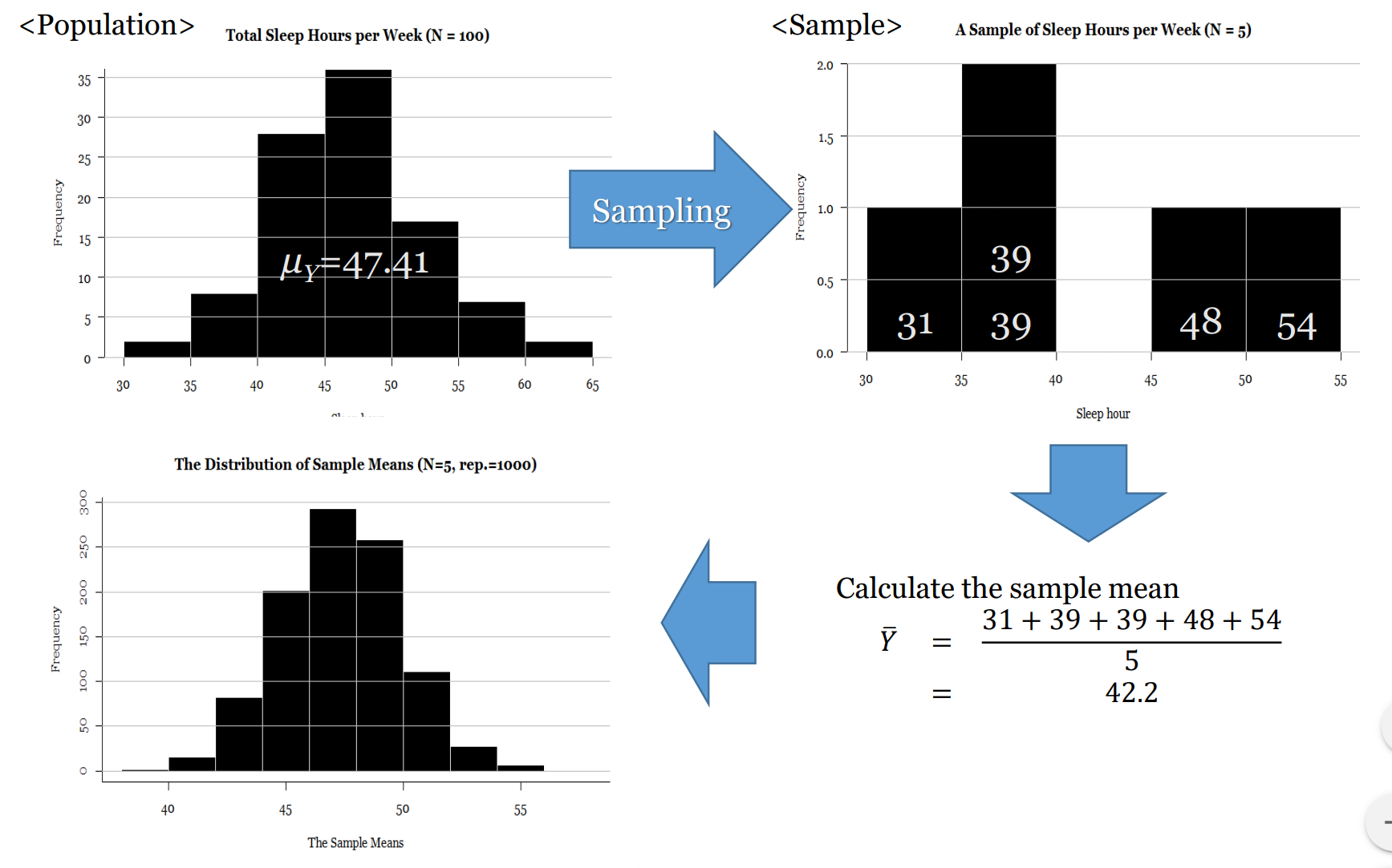
- 2.3.2 Sampling distribution: If i could do this survey 1,000 times…
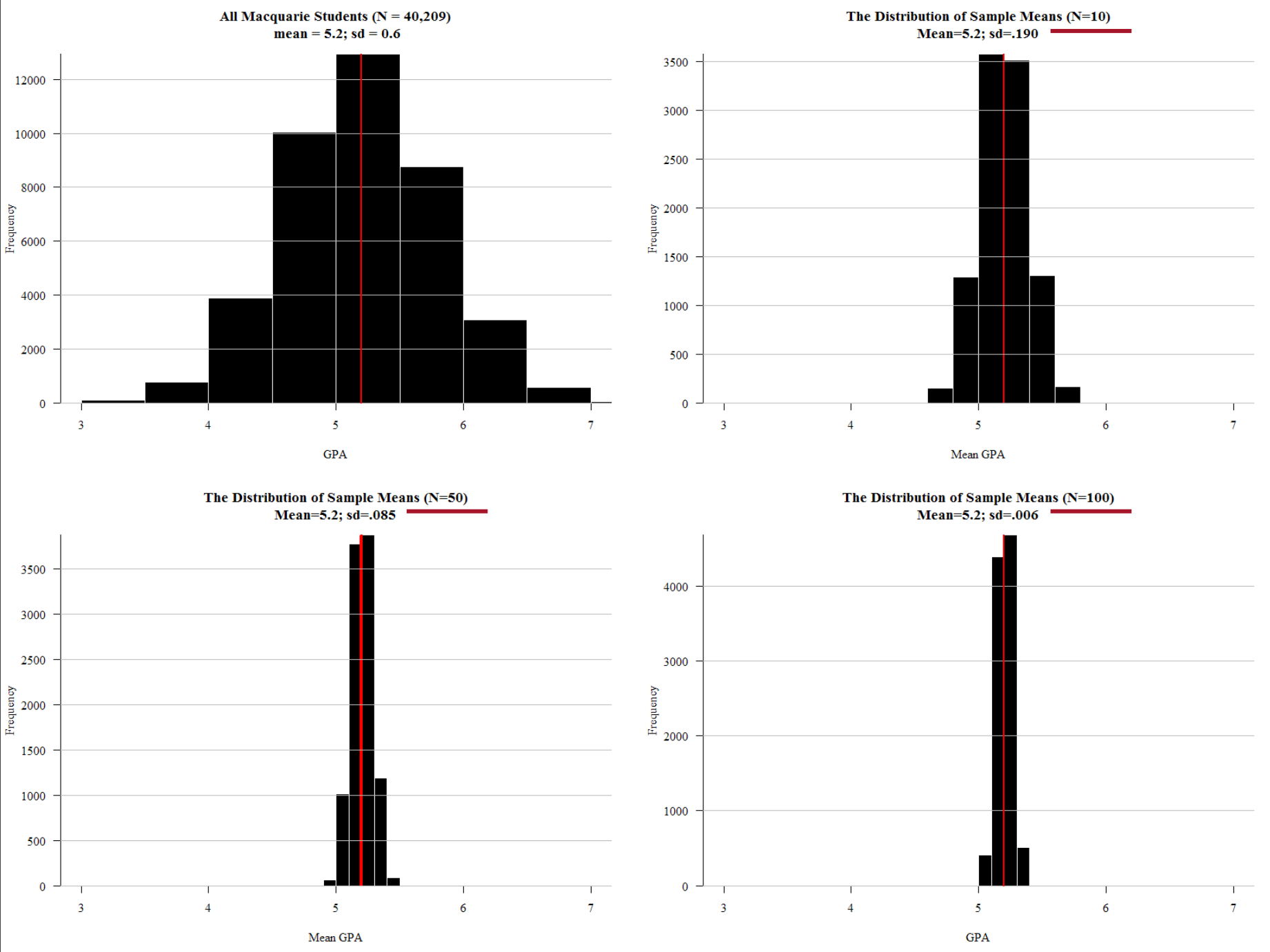
- 2.3.3 Central limit theorm: If you roll dice infinite times you always get 3.5 (on average)
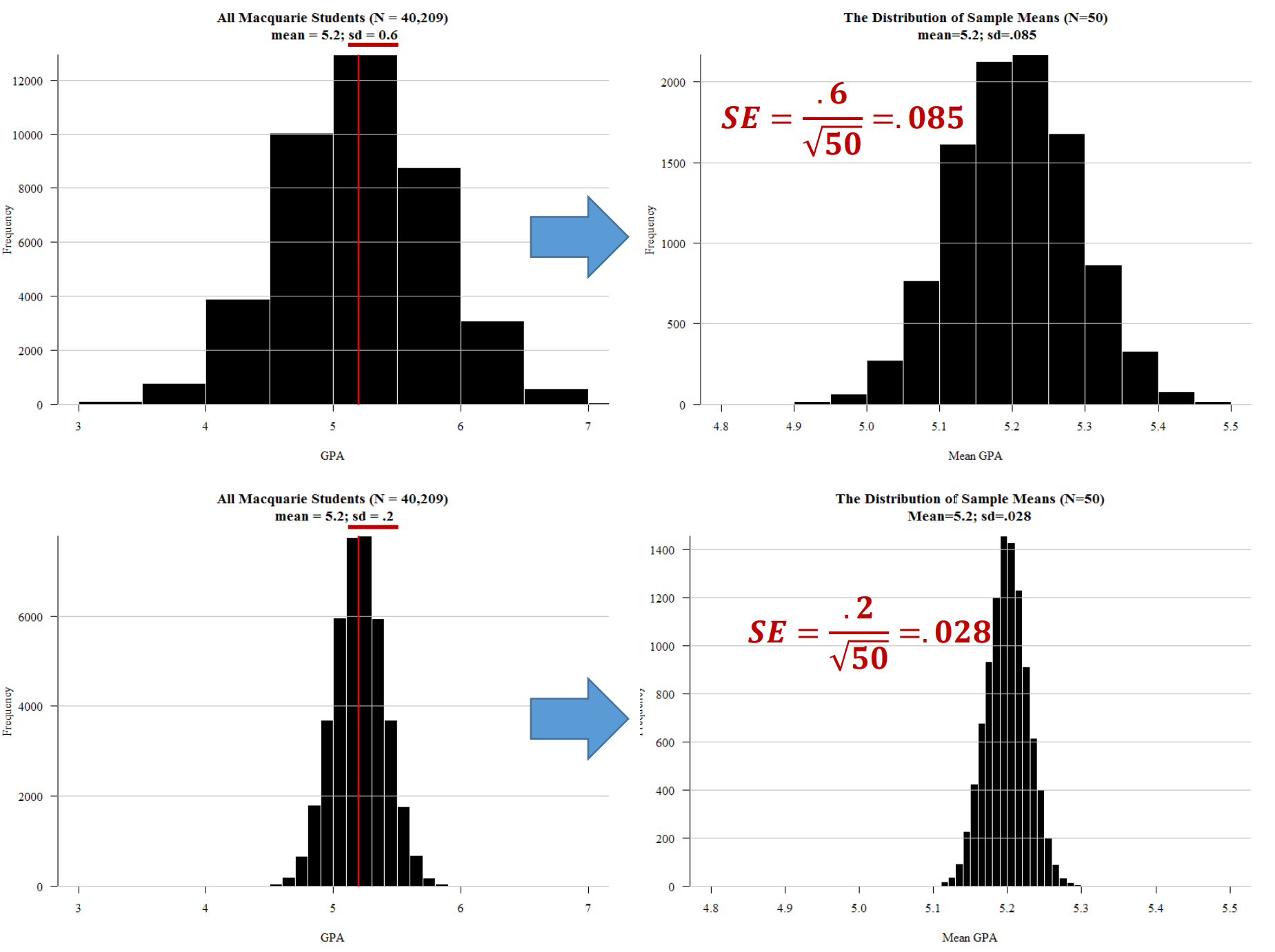
- 2.3.4 Standard error: If I repeated this survey 1,000 times… the answer would vary this much (holds up hands pretending to have caught a big fish).
- 2.3.5 Confidence interval: The population parameter is somewhere between here and here
- 2.3.6 p-value: the chance I’m wrong. The chance nothing is happening
- 2.3.7 Effect size: Does it really matter? How much?
Reading |
|
Field, A., Miles, J., and Field, Z. (2012). Discovering statistics using R. Sage publications.
|
Concepts |
|
Descriptive statistics Mean/Median/Mode (Central tendency) Standard deviation/Interquartile range (Variation/dispersion) Minimum/Maximum Percentile N (number of non-missing cases) Inferential statistics Population Population parameter Sample Sample statistic Hypothesis testing Null hypothesis Sampling distribution Central limit theorm Standard error Confidence interval p-value Effect size Bivariate inferential statistics Correlation, comparison of means, chi-squared Multivariate inferential statistics Linear and logistic regression Dimension reduction and finding categories Factor analysis, Cluster analysis |
Summary |
|
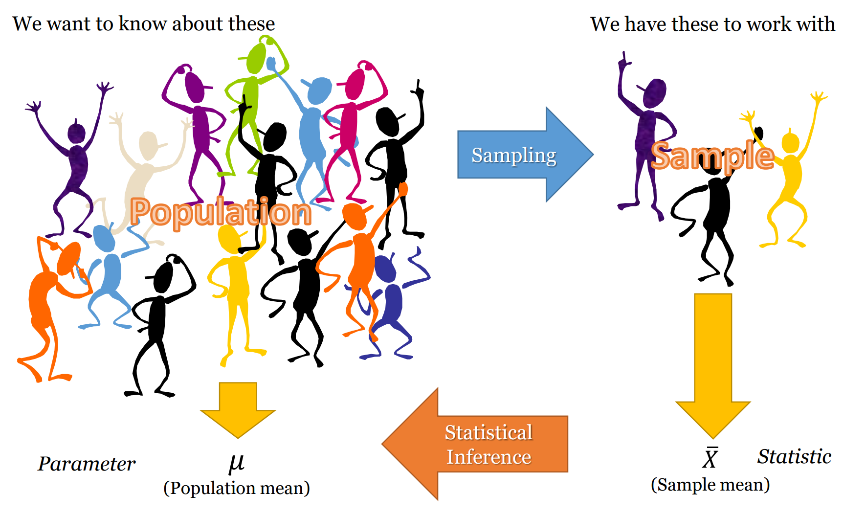
Most quantitative social science – i.e. social science that uses numbers to measure and characterise the world – uses inferential statistics to model their data and test their theories and hypotheses. At the core of inferential statistics is the idea that there is a characteristic (such as the mean number of beers drunk per week) which we are interested in measuring on population. The characteristic of the population is called a parameter. However, the population is too large to measure directly (e.g. the population of a country), so instead we need to ‘infer’ (hence the word ‘inferential’ statistics) this parameter. We infer the parameter by taking a random sample from the population. Random in this case means true randomness – all members of the population have equal chance of being in the sample. When we measure this characteristic (i.e. mean number of beers drunk per week) on the sample, we get a statistic. This sample statistic is our estimate of the population parameter. Because a sample statistic is based on a random sample, it is not a perfect reflection of the population statistic. However, because a sample is random the sample statistic has a mathematical and probabilistic relationship with the population parameter. This probabilistic relationship is expressed in statistical modelling with several different measures, such as confidence intervals, significance tests, and p-values. Most sample statistics in inferential statistics are expressed in terms of two numbers (1) a coefficient; and (2) a standard error. The coefficient represents the estimate of the population parameter (e.g. mean number of beers drunk per week in the population). The standard error is a measure of the uncertainty of this estimate. The standard error is a function of the variability of the sample and the sample size (for a mean, it is the standard deviation divided by the square root of the sample size). With most sample statistics, the major claim that we make from a model is that “There is a 95% chance that the population parameter is within +/- 1.96 standard errors of the coefficient.” This number 1.96 comes from the fact that 95% of cases in a normal distribution lie within plus or minus 1.96 standard errors of the mean of the distribution. And for most practical situations, we can assume that 1.96 is 2, and, thus, that 95% of the time the population parameter is in the range of (sample coefficient +/- 2 x standard error). So, for example, we may take a sample of 1000 Australians and find that the mean number of beers drunk per week is 3, and the standard error of this mean is 1.4. Thus, from this we can say that there is a 95% chance that the population parameter lies between 0.2 and 5.8. Or more simply, the 95% confidence interval is (0.2 – 5.8). Another way of expressing the uncertainty (or certainty) of a coefficient’s estimate of the population parameter is a significance test and p-value. In this case, we ask “What is the percentage chance of having got this sample statistic (coefficient) if the true population parameter is zero?” We use the sample coefficient, and sample standard error, and ask is the sample coefficient more than 1.96 (our magic number) standard errors away from zero? If so, then we know that the p-value (the calculated probability) of the coefficient being zero is less than 5%. When describing and modelling data, we tend to think of three main classes of statistics: univariate, bivariate, and multivariate statistics. Univariate statistics summarise single variables. The main univariate statistics include mean, median, standard deviation, frequency, minimum, maximum, quartiles and quintiles. We can use graphical representations such as histograms to illustrate univariate statistics. Bivariate statistics express the relationship between two variables. Two of the most important bivariate statistical measures are correlation coefficients (such as Pearson’s correlation coefficient), and comparisons of means. We often also use crosstabulations (crosstabs) of two variables to illustrate such data. We can represent bivariate statistics with a wide range of graphical representations, the most common being the scatterplot. Multivariate statistics model the relationship between three or more variables. Probably the canonical example of a multivariate statistics is the linear regression model, which models an outcome variable (y) as the linear product of two or more variables (e.g. university grade = hours of studying + ability to focus). |