The fourth lab session covers the following:
- How to see explanations of R codes in RStudio
- How to import an RDS file
- How to recode variables
- How to compute variables
- How to import other formats of datasets
- How to export datasets as other formats
We will use three packages for this lab. Load them using the following code:
library(dplyr)
library(sjlabelled)
library(sjmisc)
How to see explanations of R codes in RStudio
Even R experts do not know all available R codes. When they come across new R codes, they often rely on R documentation that explains them. One advantage of using RStudio is that you can easily access R documentation. Click on the tab of “Help” and type an R code you want to learn in the top right box (See Figure 1). Then, it will show R documentation about the code.
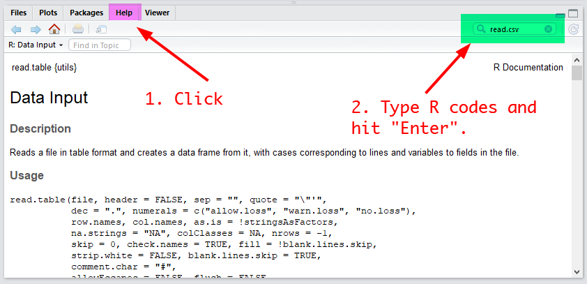
Figure 1: First Look of RStudio
The documentation provides not only detailed information on R codes but also their examples of usage. Nonetheless, reading it is not an easy task especially for those who just start learning R. However, you will get more comfortable with reading it at the end of this course..
How to import an RDS file
You saved the dataset you constructed as the RDS format in lab 3. In this lab, you are going to import it into R. Use data name <- readRDS("file-name.rds"). Then, you will see the data loaded in the tab of Environment. Run the following code.
mydata <- readRDS("mydata.rds")You will see mydata in the tab of Environment.
Recoding variables
After you start analysing survey data, you will spend most time in recoding variables. It is rare that researchers use variables as they are initially provided. Instead, researchers often customise the values of variables for their needs. This lab introduces this importnt skill of data management.
Creating a Variable of Age Groups
Suppose that we want to investigate how different age groups hold different political attitudes. However, age variable in mydata is not suitable for this purpose. Thus, we need to make a new variable of age groups using age variable. Table 1 shows the recoding scheme for this task.
| Values | Values | Labels |
|---|---|---|
| 0 - 19 | 1 | 10s |
| 20 - 29 | 2 | 20s |
| 30 - 39 | 3 | 30s |
| 40 - 49 | 4 | 40s |
| 50 - 59 | 5 | 50s |
| 60 - 69 | 6 | 60s |
| 70 - 79 | 7 | 70s |
| 80 - 89 | 8 | 80s |
| 90 or more | 9 | 90s |
To recode variables, use data name <- rec(data name, variable name, rec = "recoding scheme", append = TRUE). append = TRUE means that R will append the newly recoded variable to your dataset. For example, the following code will recode age variable in mydata and generate a new variable of age group titled age_r.
mydata <- rec(mydata, age, rec = "min:19 = 1; 20:29 = 2; 30:39 = 3; 40:49 = 4;
              50:59 = 5; 60:69 = 6; 70:79 = 7; 80:89 = 8; 90:max = 9",
              append = TRUE)
Let me explain more about “recoding scheme” in the above code. a:b means all values from a to b. For example, ‘min:19’ means all the numbers from the minimum value to 19. In the recoding scheme, we need to specify how the values of old variables are converted into the values of new variables. The left side of equal signs (=) is for the values of old variables, and the right side for the values of new variables. For example, min:19 = 1 means that all the values from the minimum value to 19 will be converted into 1. Semicolon(;) is used for separating the coding schemes of each value.
Running this code will make a new variable titled age_r. We will assign the variable and value label to this new variable by running the following code:
mydata$age_r <- set_label(mydata$age_r, label = "Age Category")
mydata$age_r <- set_labels(mydata$age_r, labels = c ("10s" = 1,
                                                     "20s" = 2,
                                                     "30s" = 3,
                                                     "40s" = 4,
                                                     "50s" = 5,
                                                     "60s" = 6,
                                                     "70s" = 7,
                                                     "80s" = 8,
                                                     "90s" = 9))
If you can’t understand the above codes, see Assigning labels and value labels to the AuSSa subsample dataset. Then, let us check the new variable by making a frequency table of it.
frq(mydata$age_r)## Age Category (x) <numeric>
## # total N=30 valid N=30 mean=4.77 sd=1.92
##
## Value | Label | N | Raw % | Valid % | Cum. %
## --------------------------------------------
## 1 | 10s | 2 | 6.67 | 6.67 | 6.67
## 2 | 20s | 1 | 3.33 | 3.33 | 10.00
## 3 | 30s | 5 | 16.67 | 16.67 | 26.67
## 4 | 40s | 5 | 16.67 | 16.67 | 43.33
## 5 | 50s | 6 | 20.00 | 20.00 | 63.33
## 6 | 60s | 6 | 20.00 | 20.00 | 83.33
## 7 | 70s | 3 | 10.00 | 10.00 | 93.33
## 8 | 80s | 1 | 3.33 | 3.33 | 96.67
## 9 | 90s | 1 | 3.33 | 3.33 | 100.00
## <NA> | <NA> | 0 | 0.00 | <NA> | <NA>Creating a new political orientation variable
Suppose that we want to use a variable political orientation that consists of three categories: left, central, and right. polorient in mydata does not fit well for this purpose because it collects more detailed information than we want. However, we can make a new variable that will serve our purpose by recoding polorient. Table 2 shows the recoding scheme for this task.
| Values | Labels | Values | Labels |
|---|---|---|---|
| 1 | Far left | 1 | Left |
| 2 | Left | 1 | Left |
| 3 | Center | 2 | Center |
| 4 | Right | 3 | Right |
| 5 | Far right | 3 | Right |
The following code will recode polorient variable in mydata and generate a new variable of political orientation titled polorient_r.
mydata <- rec(mydata, polorient, rec = "1:2 = 1; 3 = 2; 4:5 = 3", append = TRUE)Then, we will assign the variable and value label to polorient_r.
mydata$polorient_r <- set_label(mydata$polorient_r,
                                label = "3-category Political Orientation")
mydata$polorient_r <- set_labels(mydata$polorient_r, labels = c("Left" = 1,
                                                                "Center" = 2,
                                                                "Right" = 3))
The final step is to check the recoded variable.
frq(mydata$polorient_r)## 3-category Political Orientation (x) <numeric>
## # total N=30 valid N=30 mean=1.90 sd=0.99
##
## Value | Label | N | Raw % | Valid % | Cum. %
## ----------------------------------------------
## 1 | Left | 16 | 53.33 | 53.33 | 53.33
## 2 | Center | 1 | 3.33 | 3.33 | 56.67
## 3 | Right | 13 | 43.33 | 43.33 | 100.00
## <NA> | <NA> | 0 | 0.00 | <NA> | <NA>Renaming variables
The name of recoded variables are automatically assigned as ‘variable name_r’. However, you may want to change variable names. In this case, use ‘data name <- var_rename(data name, current name = "new name", ...)’ For example, the following code will change age_r, polorient_r and class_r into age_gr, polorient_3 and class_3, respectively.
mydata <- var_rename(mydata, age_r = "age_gr", polorient_r = "polorient_3",
class_r = "class_3")Computing variables
Another way to make a new variable is to compute variables. It is useful especially when the relationship between old and new variables can be expressed in mathematical equations.
For example, let us make a variable of birth year. The relationship between birth year and age is \(birth year = 2020 - Age\). Using this equation, we can create a variable of birth year by data name <- data name %>% mutate(new variable name = Equation). In this code, %>% is called ‘pipes’, which means ‘after then’. mutate() is the function for making a new variable. Thus, the meaning of code is: 1) use data name, 2) after then, make new variable name using the Equation, 3) data name will include this newly generated variable. The following code will also assign the variable label.
mydata <- mydata %>%
mutate(b_year = 2020 - mydata$age)
mydata$b_year <- set_label(mydata$b_year, label = "Year of Birth")
mydata$b_year## [1] 1954 1948 1961 2000 1952 1944 1959 1930 1956 1981 1963 1973 1964 1969 1986
## [16] 2002 2002 1990 1955 1985 1976 1980 1963 1980 1961 1938 1976 1990 1943 1960
## attr(,"label")
## [1] "Year of Birth"Removing variables
In case you want to remove unnecessary variables from data, use ‘the following code remove_var() function. The following code will remove b_year. The code is data name <- data name %>% remove_var(variable name). You can remove multiple variables by’remove_var(var 1, var 2, var 3, var 4, ...)’.
mydata <- mydata %>%
remove_var(b_year)The code means: 1) choose mydata, and then(%>%) 2) remove a variable of b_year.
Saving your dataset again
Save your dataset again. This time I use a different file name (I saved it as “mydata.rds” in lab 3) so that I can keep all the dataset files I have worked on so far.
saveRDS(mydata, file = "mydata-2.rds")How to import other formats of datasets
Public datasets are not provided as an R-compatible format. Normally, they are offered in either SPSS or STATA formats. To import SPSS-format datasets (.sav), use the read_spss() function. Click on this. You will be able to download an example SPSS dataset. Put this downloaded file in your working folder and run the following code:
spss <- read_spss("spss-example.sav")To import STATA-format datasets (.dta), use the read_stata() function. Click on this. You will be able to download an example STATA dataset. Put the downloaded file in your working folder and run the following code:
stata <- read_stata("stata-example.dta")
Lab 4 Participation Activity |
|
No Lab Participation Activity this week because I want you to spend more time for preparing for the online quiz. But this lab provides essential knowledge for manipulating variables. Without understanding it you won’t be able to complete the R Analysis Tasks. Therefore, I recommend that you review Lab 4 thoroughly after you have completed the online quiz. |
The R codes you have written so far look like:
################################################################################
# Title: Lab 4
# Course: SOCI8015 & SOCX8015
# Date: 22/03/2021
################################################################################
# Load packages
library(dplyr)
library(sjlabelled)
library(sjmisc)
# Import an RDS dataset
mydata <- readRDS("mydata.rds")
# Recode variables
## Create age groups
mydata <- rec(mydata, age, rec = "min:19 = 1; 20:29 = 2; 30:39 = 3; 40:49 = 4;
50:59 = 5; 60:69 = 6; 70:79 = 7; 80:89 = 8; 90:max = 9",
append = TRUE)
mydata$age_r <- set_label(mydata$age_r, label = "Age Category")
mydata$age_r <- set_labels(mydata$age_r, labels = c ("10s" = 1,
"20s" = 2,
"30s" = 3,
"40s" = 4,
"50s" = 5,
"60s" = 6,
"70s" = 7,
"80s" = 8,
"90s" = 9))
frq(mydata$age_r)
## Create 3-category political orientation
mydata <- rec(mydata, polorient, rec = "1:2 = 1; 3 = 2; 4:5 = 3", append = TRUE)
mydata$polorient_r <- set_label(mydata$polorient_r,
label = "3-category Political Orientation")
mydata$polorient_r <- set_labels(mydata$polorient_r, labels = c("Left" = 1,
"Center" = 2,
"Right" = 3))
frq(mydata$polorient_r)
## Create 3-category social class
mydata <- rec(mydata, class, rec = "1:2 = 1; 3:5 = 2; 6 = 3", append = TRUE)
mydata$class_r <- set_label(mydata$class_r,
                            label = "3-category Social Class")
mydata$class_r <- set_labels(mydata$class_r, labels = c("Lower class" = 1,
                                                        "Middle class" = 2,
                                                        "Upper class" = 3))
frq(mydata$class_r)
# Rename variables
mydata <- var_rename(mydata, age_r = "age_gr", polorient_r = "polorient_3",
                     class_r = "class_3")
# Compute variables
mydata <- mydata %>%
  mutate(b_year = 2020 - mydata$age)
mydata$b_year <- set_label(mydata$b_year, label = "Year of Birth")
mydata$b_year
# Remove variables
mydata <- mydata %>%
  remove_var(b_year)
# Save the data file
saveRDS(mydata, file = "mydata-2.rds")
# Import other formats of datasets
## Import SPSS datasets
spss <- read_spss("spss-example.sav")
## Import STATA datasets
stata <- read_stata("stata-example.dta")