0. Code to run to set up your computer.
# Update Packages
update.packages(ask = FALSE, repos='https://cran.csiro.au/', dependencies = TRUE)
# Install Packages
if(!require(dplyr)) {install.packages("dplyr", repos='https://cran.csiro.au/', dependencies=TRUE)}
if(!require(sjlabelled)) {install.packages("sjlabelled", repos='https://cran.csiro.au/', dependencies=TRUE)}
if(!require(sjmisc)) {install.packages("sjmisc", repos='https://cran.csiro.au/', dependencies=TRUE)}
if(!require(sjstats)) {install.packages("sjstats", repos='https://cran.csiro.au/', dependencies=TRUE)}
if(!require(sjPlot)) {install.packages("sjPlot", repos='https://cran.csiro.au/', dependencies=TRUE)}
if(!require(lm.beta)) {install.packages("lm.beta", repos='https://cran.csiro.au/', dependencies=TRUE)}
# Load packages into memory
base::library(dplyr)
base::library(sjlabelled)
base::library(sjmisc)
base::library(sjstats)
base::library(sjPlot)
base::library(lm.beta)
# Turn off scientific notation
options(digits=3, scipen=8)
# Stop View from overloading memory with a large datasets
RStudioView <- View
View <- function(x) {
if ("data.frame" %in% class(x)) { RStudioView(x[1:500,]) } else { RStudioView(x) }
}
# Datasets
# Example 1: Crime Dataset
lga <- readRDS(url("https://methods101.com/data/nsw-lga-crime-clean.RDS"))
# Example 2: AuSSA Dataset
aus2012 <- readRDS(url("https://mqsociology.github.io/learn-r/soci832/aussa2012.RDS"))
# Example 3: Australian Electoral Survey
aes_full <- readRDS(gzcon(url("https://mqsociology.github.io/learn-r/soci832/aes_full.rds")))
# Example 4: AES 2013, reduced
elect_2013 <- read.csv(url("https://methods101.com/data/elect_2013.csv"))1. Regression Diagnostics
Any model is only valid if the assumptions it is based on are true.
This is true for linear regression models too.
For linear regression models, there are really two very different parts:
- the coefficients: these tell us the slope of the relationship between the dependent (DV) and independent (IV) variables. For example, 1 conflict at work (IV) causes a 10 mm Hg increase in my blood pressure(DV))
- the standard error of the coefficients: These tell us the range within with the true POPULATION PARAMETER for coefficient is likely to sit. Fore xample, we might have a standard error of the coefficient of 4 mm Hg, which means 95% of the time we would expect that the true population coefficient is between 2 mm Hg and 18 mm Hg (i.e. the coefficient +/- 2 * standard error).
For each of these parts of the model, there are different assumptions.
1.1 Assumptions about coefficient
In general, the assumptions that underly the coefficients are about the proper fit (or) otherwise of the coefficients to the sample (i.e. does the line estimating the relationship between the IV and DV pass through the middle of the points on a graph).
1.2 Assumptions about standard error of coefficent
In contrast, the assumptions related to the standard error are about the ability of the model to be generalised to the larger population: these tend to be about whether the standard errors properly reflect the likely variation (or non-variation) in the value of the population parameter.
For each of the various assumptions, there are three questions to ask
- ASSUMPTION: what is the assumption;
- TEST: how do we test the assumption - also called a diagnostic test - ; and
- TREATMENT: how do we fix or address this problem if we find it.
2. Diagnostic tests
2.1 Outliers
2.1.1 Theory
One basic ASSUMPTION of all models is that there are very few outliers. An outlier is a case (a unit of analysis - e.g. survey respondent) whose value on the outcome variable (dependent variable) is poorly explained by the explanatory variables (independent variables).
The reason outliers are a problem is that they show that the model is a bad explanation of the data. Basically it’s a bad model.
How do we TEST if we have outliers?
Unexplained variation in dependent variable = residual
We look to see if there is a large amount of unexplained value of the dependent variable for any particular case. Remember that for a linear regression model the explained part of the dependent variable is the value of the dependent variable as predicted by all the independent variables.
For example, say estimate a model of likelihood of voting (from 1 to 5) as predicted by political knowledge (measured from 0 to 10 on quiz).
Suppose that the estimated model is:
\(\begin{aligned} \text{likelihood_vote} = &0.5*\text{pol_knowledge} \\ \end{aligned}\)
And suppose we have a person called “Tom” with:
- a likelihood of voting of “1”, and
- a political knowledge of 6.
Tom’s predicted likelihood_vote would be:
6*0.5 = 3.
However, his actual likelihood is 1.
The unexplained part of Tom’s vote is
3 - 1 = 2.
We call this unexplained part (2) of outcome variable the residual.
Outliers are identified by the fact that they have very large residuals.
Standardised units of analysis
Now it turns out that since variables are measured in many different units of analysis, we need to standardise the units of analysis of residuals so that they have some universal unit.
And you will remember from previous classes the main way we standardise and create universal units is by dividing values by the standard deviation of those values so that a case with a value of 1 is is known to have residuals exactly one standard deviation away from the coefficient.
So the measure we use to TEST for outliers is standardised residuals.
We calculate the value of this on all the cases in our dataset, and then we look at the proportion of those that lie outside what you would expect to find by chance.
And how do we do that? We look to see how many have standardized residuals that are different from those expected in a normal distribution.
And this test is quite straightforward.
We expect
- That 95% of cases have standardized residuals of between +/- 1.96;
- That 99% of cases have standardized residuals of between +/- 2.58; and
- That 95% of cases have standardized residuals of between +/- 3.29.
2.1.2 R Script
Let’s look at how we do this in R
First we need to run a model. In this case we run a simple model of political knowledge, with one predictor: interest in politics.
model_1 <- lm(elect_2013$pol_knowledge
              ~ elect_2013$interest_pol
              + elect_2013$highest_qual
              + elect_2013$age_cat
              + elect_2013$female
              + elect_2013$tertiary_ed
              + elect_2013$income)
If you want to see this model’s coefficients, then you can run:
summary(model_1)##
## Call:
## lm(formula = elect_2013$pol_knowledge ~ elect_2013$interest_pol +
## elect_2013$highest_qual + elect_2013$age_cat + elect_2013$female +
## elect_2013$tertiary_ed + elect_2013$income)
##
## Residuals:
## Min 1Q Median 3Q Max
## -7.785 -1.747 0.031 1.735 7.957
##
## Coefficients:
## Estimate Std. Error t value Pr(>|t|)
## (Intercept) 5.02773 0.24318 20.67 <2e-16 ***
## elect_2013$interest_pol -1.38298 0.05418 -25.53 <2e-16 ***
## elect_2013$highest_qual 0.03003 0.01934 1.55 0.12
## elect_2013$age_cat 0.35984 0.02931 12.28 <2e-16 ***
## elect_2013$female -0.67519 0.08157 -8.28 <2e-16 ***
## elect_2013$tertiary_ed 1.15641 0.09680 11.95 <2e-16 ***
## elect_2013$income 0.06613 0.00717 9.22 <2e-16 ***
## ---
## Signif. codes: 0 '***' 0.001 '**' 0.01 '*' 0.05 '.' 0.1 ' ' 1
##
## Residual standard error: 2.37 on 3497 degrees of freedom
## (451 observations deleted due to missingness)
## Multiple R-squared: 0.319, Adjusted R-squared: 0.317
## F-statistic: 272 on 6 and 3497 DF, p-value: <2e-16Next we construct a new data frame which will hold the variables from our model.
I’ve given it the name ‘diagnostics’, but you could call it anything.
diagnostics <- model_1$modelYou can view this data frame by double clicking on it in the top right corner of your RStudio window.
Next we want to put the main residuals into the new data frame. The most important of these is the third set - the standardised residuals
diagnostics$fitted.values <- model_1$fitted.values
diagnostics$residuals <- model_1$residuals
diagnostics$standardized.res <- rstandard(model_1)
diagnostics$student.res <- rstudent(model_1)
Now we need to run the tests.
2.1.2.1 Test 1: 95% cases with standardized residuals < +/- 1.96
Remember that the first test was 95%+ cases with standardised residuals between +/- 1.96. Another way to say this is “No more than 5% of cases with absolute value of standardised residual of greater than 1.96”.
How many cases is 5% of cases in your dataset?
We can just measure the length of a variable to get the number of cases in our dataset and then multiply that by 0.05
MAXIMUM CASES EXPECTED:
length(diagnostics$standardized.res)*0.05## [1] 175?o how many cases in our dataset have an absolute value of the standardised residual of > 1.96:
ACTUAL NUMBER OF CASES IN THIS DATASET:
sum(abs(diagnostics$standardized.res) > 1.96)## [1] 140The equation above tells us it is 150, which is less that 197.1, and thus less than 5%.
We can repeat this with the other two tests
2.1.2.2 Test 2: 99% cases with SR < +/- 2.85
“No more than 1% of cases with absolute value of standardised residual of greater than 2.58”.
MAXIMUM CASES EXPECTED:
length(diagnostics$standardized.res)*0.01## [1] 35ACTUAL NUMBER OF CASES IN THIS DATASET:
sum(abs(diagnostics$standardized.res) > 2.58)## [1] 202.1.2.2 Test 3: 99.9% cases with SR < +/- 3.29
“No more than 0.1% of cases with absolute value of standardised residual of greater than 3.29”.
MAXIMUM CASES EXPECTED:
length(diagnostics$standardized.res)*0.001## [1] 3.5ACTUAL NUMBER OF CASES IN THIS DATASET:
sum(abs(diagnostics$standardized.res) > 3.29)## [1] 12.2 Influential Cases
2.2.1 Theory
While outliers are cases that are not explained by a model, influential cases are those that disproportionately effect the coefficients of the model.
We can think of the influence of an individual case (e.g. one person who does our survey) by asking how much does the coefficient for a predictor variable in a model change when this one case is dropped out of the dataset.
There are many different measures of influential cases, and it is beyond this course to explain how these are calculated and exactly what they mean. For our purposes, the key things to understand are (1) what tests we should run; and (2) how to judge whether our model passes these tests or not. In addition we may want to be able to answer (3) what should we do if our data fails the test.
The two measures of influential cases we are going to look at are:
- Cook’s Distance, and
- Leverage.
Cook’s Distance is calculated on all cases (e.g. respondants) and a case is considered a problem - i.e. too influential - if it has a Cook’s Distance greater than 1.
Leverage is also calculated on all cases.
There are different rules of thumb about what level of leverage is problematic.
More than two or three times the average leverage is generally thought of as a problem. The average leverage, however, varies with the number of preditors in a model, and the number of observations in a dataset, so we need to calculate the maximum leverage for each model.
The forumula is:
\(\begin{aligned} \text{MAXIMUM LEVERAGE} = &3*(k+1)/n \\ \\ \text{Where:}\\ k=&\text{coefficents in model}\\ n=&\text{observations}\\ \end{aligned}\)
2.2.2 R Script
The various measures of influential cases can be calculated and stored with the following commands:
diagnostics$cooks.distance <- cooks.distance(model_1)
diagnostics$dfbeta <- dfbeta(model_1)
diagnostics$dffits <- dffits(model_1)
diagnostics$leverage <- hatvalues(model_1)
diagnostics$covariance.ratios <- covratio(model_1)
We can then check the maximum Cook’s Distance (which should be > 1) with this command:
max(diagnostics$cooks.distance)## [1] 0.00695And then we can check that the maxmimum leverage is below the prescribed level of:
\(\begin{aligned} \text{MAXIMUM LEVERAGE} = &3*(k+1)/n \\ \end{aligned}\)
k <- length(model_1$coefficients) - 1
n <- length(diagnostics)
MAXIMUM LEVERAGE ALLOWED:
((k + 1)/n)*3## [1] 1.31MAX LEVERAGE IN THIS DATA:
max(diagnostics$leverage)## [1] 0.006452.3 Multicollinearity
2.3.1 Theory
Another problem which a model can have is that the predictor variables (independent variables) are highly collinear.
Some level of collinearity is to be expected. However, when the correlation between variables is extreme - like 0.8 or 0.9 or higher - then this collinearity can undermine the quality of a linear regression model.
The problem is that such colinearity tends to inflate - i.e. artificially increase - the standard errors of coefficients. And if the standard errors are artificially larger, then predictor variables that are ACTUALLY statistically significant (i.e. p value < 0.05 and/or 95% confidence interval does not include zero), will APPEAR to be not significant.
The main way that we check for multicollinearity in a regression model is with the Variance Inflation Factor (VIF) (and it’s inverse, which is called Tolerance).
The rule of thumb is that the highest VIF for any coefficient in the model should be less than 10, and ideally less that 5 or even 2.5.
Another rule of thumb is that the average VIF should not be substantially greater than 1. However, from what I can find in a casual search, it’s not clear exactly what ‘substantially greater than 1’ means. My reading is that the average should be below ~ 2 or 3.
2.3.2 R Script
To measure Variance Inflation Factor (VIF) we need to install and load the “car” package
if(!require(car)) {install.packages("car", repos='https://cran.csiro.au/', dependencies=TRUE)}
library(car)
The VIF for each variable in a model is given by this command:
vif(model_1)## elect_2013$interest_pol elect_2013$highest_qual elect_2013$age_cat
## 1.15 1.09 1.24
## elect_2013$female elect_2013$tertiary_ed elect_2013$income
## 1.03 1.24 1.24if you don’t want to read and look for the maximum VIF, then you can use this command and check that the results is below the threshold of 10 (or more conservatively 5).
max(vif(model_1))## [1] 1.24And you can check the mean VIF with this command:
mean(vif(model_1))## [1] 1.17To illustrate the relevance of VIF and also of centring interaction effects, we will compare the VIF diagnostics for two different interaction effects (we will learn more about these next week).
Below I’ve simply pasted the two linear regression models, and then run the three diagnostics. Remember that the maximum VIF should be below 10, and ideally below 5 or even 4. Run the code and interpret the results.
model_normal <- lm(elect_2013$likelihood_vote ~
                elect_2013$internet_skills*elect_2013$age_18_24)

elect_2013$centred.internet_skills.x.age_18_24 <-
  (elect_2013$internet_skills-
     mean(elect_2013$internet_skills, na.rm = TRUE))*(elect_2013$age_18_24-mean(elect_2013$age_18_24, na.rm = TRUE))

model_centred <- lm(elect_2013$likelihood_vote ~
                elect_2013$internet_skills +
                elect_2013$age_18_24 +
                elect_2013$centred.internet_skills.x.age_18_24)

car::vif(model_normal)
## elect_2013$internet_skills
## 1.08
## elect_2013$age_18_24
## 13.02
## elect_2013$internet_skills:elect_2013$age_18_24
## 13.26car::vif(model_centred)## elect_2013$internet_skills
## 1.09
## elect_2013$age_18_24
## 2.94
## elect_2013$centred.internet_skills.x.age_18_24
## 2.80max(car::vif(model_normal))## [1] 13.3max(car::vif(model_centred))## [1] 2.94mean(car::vif(model_normal))## [1] 9.12mean(car::vif(model_centred))## [1] 2.282.4 Homeoscedasticity
2.4.1 Theory
The residuals - which are the difference between the predicted value (the value predicted by our model) of the dependent variable, and the actual observed value - should be distributed randomly and distributed with the same variance at all levels of the (predicted) dependent variable.
Why does this matter?
It matters because when there is heteroscedasticity (i.e. not homoscedasticity), the variance - and therefore standard errors - are underestimated, making inference from the model to a population unsound.
2.4.1 R Script
The simplest way to test for homoscedasticity is to use a built in function in R, where you simply call the command ‘plot()’ and place the regression model data in the function.
Note that when you run this command, R will say to you in the console window:
“Hit
When you hit
plot(model_1)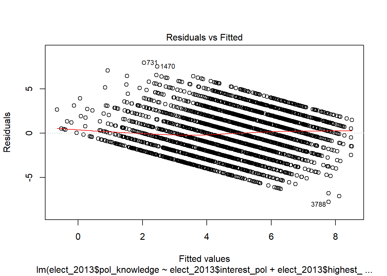
This first plot is the most important. It is the plot of the residuals against the fitted values of the dependent variable.
The general advice for evaluating this plot is that the values should be evenly distributed across the different values of the fitted values.
Heteroscedasticity normally manifests as a ‘funnel’ shape of the residuals, with small variance in residuals for low fitted values, and large residuals for high fitted values.
In practice, the plots which one sees are often hard to evaluate - especially for someone who is not an expert and experienced regression modeller and statistician.
In general I would recommend running this test and then referring to the textbook (Field et al. 2012: section 7.9.5), and websites such as this:
http://www.contrib.andrew.cmu.edu/~achoulde/94842/homework/regression_diagnostics.html
2.5 Independence of Errors
2.5.1 Theory
Another assumption we can test is independence of errors. This is not normally a problem unless one has samples on the same people (e.g. in time series data) or some strong sequencing effect caused by sampling (e.g. you sample people who are friends or who are living in close geographic proximity).
A test for independence of errors is the Durbin Watson Test. The statistic for this test should be more than 1 and less than 3, and the p-value for the test should be greater than 0.05.
Note that because this test is a sequential test it is dependent on the sort order of the data.frame. If you change the sort order of the data.frame, or you randomise the order of cases, then the DW test will be different, and probably show independence of errors (even if this is untrue)
2.5.2 R Script
This is the command for running the D-W Test. Remember that the D-W Statistic should be between 1 and 3, and the p-value of the test should be greater than 0.05.
durbinWatsonTest(model_1)## lag Autocorrelation D-W Statistic p-value
## 1 0.0061 1.99 0.744
## Alternative hypothesis: rho != 02.6 Normal Distribution of Errors
2.6.1 Theory
One last assumption that we will test is the assumption that residuals are normally distributed.
We have already tested some aspects of the normal distribution when we tested for outliers (2.1).
However, a lack of outliers is only one aspect of a normal distribution. A distribution could - and often does - lack outliers but still not be normal. It could be, for example:
- very skewed with the values are mostly at one end of the range (e.g. a survey question where most people say ‘strongly agree’), or
- they could be bifucated with two peaks (e.g. heights of a group of parents and children on a hike).
In our case, we are not looking at a variable directly but rather the residuals of a variable. Nonetheless, the distribution of residuals has the potential, like any distribution, to not be normally distributed in many different ways.
One way to test for all these different possibilities is to just visually inspect the residuals. And we do this by simply visually inspecting the histogram of the standardised residuals.
The test we apply is rather rough, but is essentially: Does it look like a symetrical bell curve, centred on a standardised residual of zero?
If the answer is yes - more or less - then we are generally satisfied that the assumption holds.
There are more advanced tests - for measuring skewness, for example - but these are generally not used unless there is a very specific reason.
2.6.2 R Script
What do we visually inspect the standardised residuals? The command is simply:
hist(diagnostics$standardized.res)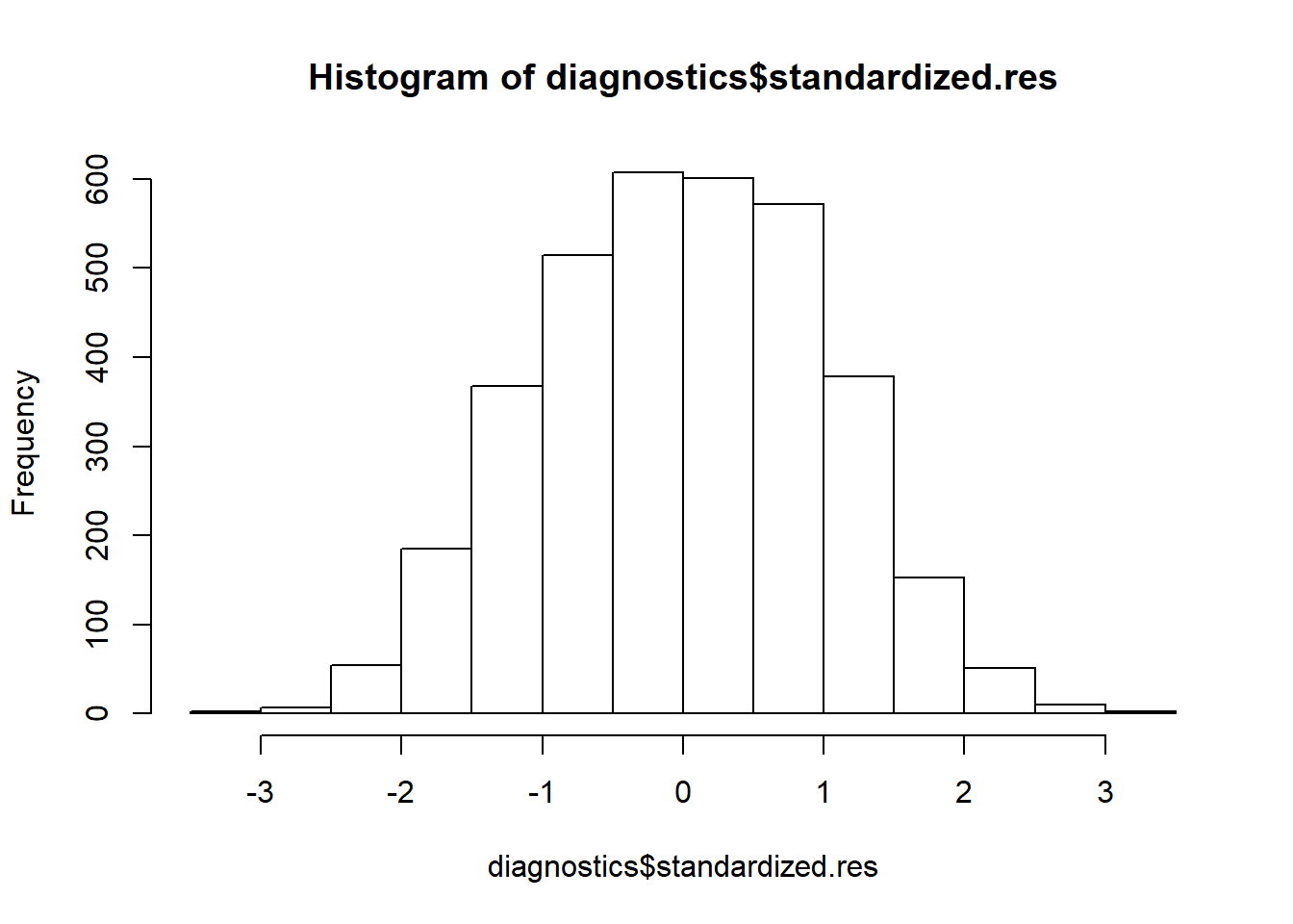
In this case the residuals look normally distributed
However, we can come up with an example that violates this assumption of normality. Run the following code and inspect the standardised residuals.
model_2 <- lm(elect_2013$likelihood_vote
              ~ elect_2013$pol_knowledge)
diag2 <- model_2$model
diag2$standardized.res <- rstandard(model_2)
hist(diag2$standardized.res)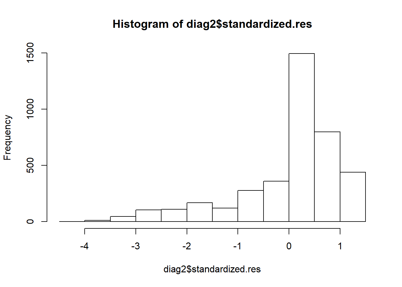
The visual inspection of the histogram shows a serious problem with skewness. One reason this happens because the dependent variable - likelihood_vote - is so skewed. Regardless, the point here is that there are models which fail this test.
2.7 What to do when assumptions are violated?
2.7.1 Theory
What do we do if our data or model violates one or more of these assumptions?
There are lots of different techniques and tricks that can be used to address these problems. I will try to list some of the most common here:
- Add more or different independent variables
- Transform your dependent variable (e.g. taking the cubed root of your dependent variable can often transform it to be more normally distributed)
- Bootstrap your standard errors: This is a technique for estimating the standard errors through simulations - rather than calculation - and allows standard errors to be estimated for very ‘non-conventional’ or ‘extreme’ distributions.
- Use a different type of regression model: It turns out that some models - such as logit - are more robust and make fewer assumptions. And other models - such as poission models - assume different distributions that might be more appropriate for your data.
Applying all these techniques is beyond this week’s class, but we will deal with many of these ideas over the course of the semester.