In the workshop 9, we will use the 2012 Australian Survey of Social Attitudes (AuSSA). Open the 2012 AuSSA for this workshop. The data file is in your SSCI2020 folder.
This workshop introduces how to produce crosstabs and how to conduct the Chi-square test of Independence.
Crosstabs and Chi-square
We often use a frequency table to describe a categorical variable (such as a nominal or ordinal variable). What if you want to describe a relationship between two categorical variables? In this case, we need a special type of tables called cross-tabulation (or crosstab for short).
In a crosstab, the categories of one variable determine the rows of tables, and those of the other variable determine the columns. The cells of tables contain the frequency that a particular combination of independent and dependent categories occurs.
Suppose that we are investigating whether there is an association between gender of respondents (sex) and attitudes toward traditional gender roles (hubbywk). hubbywk measures the extent to which respondents agree or disagree with the statement that a man’s job is to earn money, and a woman’s job is to look after the home and family. We hypothesise that gender would influence the attitude toward traditional gender roles. Therefore, we think of gender as an independent variable and the attitude as a dependent variable.
To create a crosstab, click Analyze > Descriptive Statistics > Crosstabs. In the box of Crosstabs, 1) move a dependent variable (in this case hubbywk) to the box of Row(s) and 2) an independent variable (in this case sex) to the box of Column(s). 3) Click Statistics. Make sure that dependent variables should be in the box of Row(s) and independent variables in the box of Column(s). Otherwise, your crosstabs will not be displayed correctly.
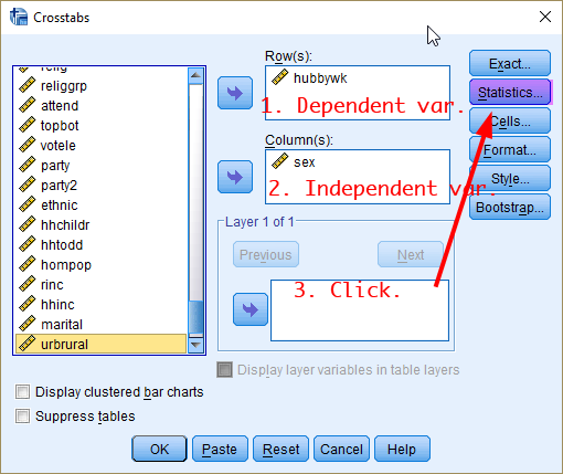
Figure 1: <Figure 1>
In the box of Crosstabs: Statistics, 1) tick the box of Chi-square. Then 2) Click Continue.
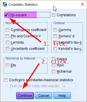
Figure 2: <Figure 2>
In the previous window (<Figure 1>), click Cells. In the box of Crosstabs: Cell Display, 1) tick the box of Observed under Counts and 2) the box of Column under Percentages (which will show the column percentages).
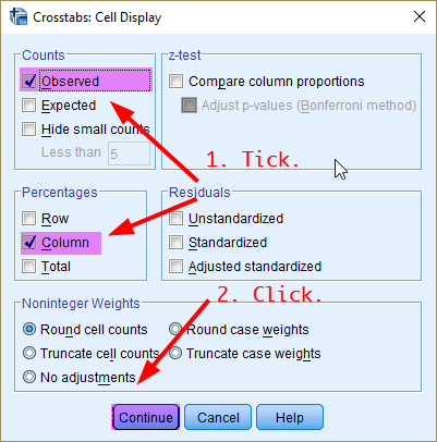
Figure 3: <Figure 3>
In the previous window (<Figure 1>), click OK. This will show a crosstab and its Chi-square statistic.
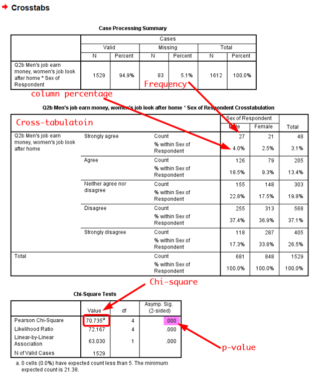
Figure 4: <Figure 4>
In <Figure 4>, the first table shows a summary of valid cases and missing cases. The second table shows the crosstab of attitudes toward traditional gender roles by gender. Each cell shows frequencies and their column percentages. Note that column percentages are computed within a specific column (in this case, within a category of gender). The third table displays a Chi-square statistic and its associated p-value.
Based on <Figure 4>, how would you describe the association between gender and attitudes toward traditional gender roles? Do you think this association is statistically significant? And explain why? If you are not sure, please see week 10 lecture slides.
General Guidelines for Recoding Variables
In this section, I would like to give general guidelines for recoding variables. You have so far recoded many variables over this semester. But I found many students are still confused at how to recode variables. When you analyse data, you need to recode variables into new one which should match well with your research idea. Thus, recoding variables appropriately is essential for completing your research project. Every time you want to recode variables, following the steps below. Make sure that this guideline is not limited to this workshop. It is a general guideline that can be applied to any case when you recode variables.
When you examine bivariate association using a crosstab, it can be very daunting if your categorical variable has too many categories, or you are using a continuous variable. The best solution for this case is to recode variables (e.g. combining similar categories) so that you can have reduced numbers of categories (but the reduced categories should be still theoretically meaningful).
In this week workshop activity (Workshop Activity 9), you will use Education, Age, and Class as independent variables. Education (degree) is an ordinal variable with seven categories, but you do not need such detailed categories when you examine the relationship using crosstabs. Also, Age and Class are continuous variables, and thus categorising these three variables is necessary for the crosstabulation analysis.
First, generate the frequency table of the variable you want to recode. When you recode a variable, it is always good to create a frequency table of the variable you want to recode. This will give you an idea of whether and how you need to recode variables. For example, <Figure 5> shows the frequency table of degree.
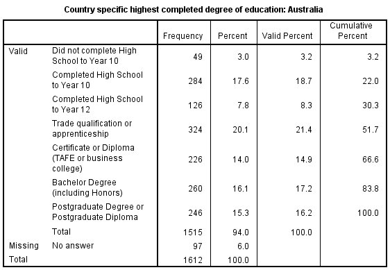
Figure 5: <Figure 5>
Second, make a recoding scheme for your new variable. <Figure 5> tells you that there are seven categories in degree. How would you recode this variable? There is no hard and fast rule for which categories should be combined. But there are two rules of thumb which could help you to make a decision.
Sometimes, there exist theoretically justifiable breaking points in the response categories. For example, when you try to reduce the categories in degree, creating three categories-“high school degree or less than high school degree”, “vocational education & training”, and “bachelor degree or post-graduate degree”)- makes sense because each degree in this categorisaion impacts the life course in a qualitatively different way.
The second rule considers empirical advantage of having sufficient numbers of cases in each category in a newly recoded variable. This is because a very small number of cases in any category can hinder Chi-square test from obtaining statistically robust outcomes. For example, when you look at degree, the number of those who did not complete high school seems to be too small to be treated as one independent category. But if this group is theoretically important to you, you can treat this group as one separate category (Theoretical importance is more important than empirical consideration, almost always!).
All these rules considered, the following recoding scheme of <Table 1> is proposed. To make a recoding scheme like this table by yourself, first you need to check specific values that are assigned to each category. You can do so by clicking the Values column of variables in the tab of Variable View as in <Figure 6> or looking at the codebook of your dataset.
| Values | Labels | Values | Labels |
|---|---|---|---|
| 1 | Did not complete High School to Year 10 | 1 | High school or less |
| 2 | Completed High School to Year 10 | ||
| 3 | Completed High School to Year 12 | ||
| 4 | Trade qualification or apprenticeship | 2 | Vocational Education & Training (VET) |
| 5 | Certificate or Diploma (TAFE or business college) | ||
| 6 | Bachelor Degree (including Honors) | 3 | University or more |
| 7 | Postgraduate Degree or Postgraduate Diploma |
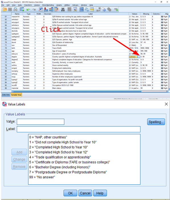
Figure 6: <Figure 6>
- Provide your recoding scheme to SPSS using Recode into Different Variables.
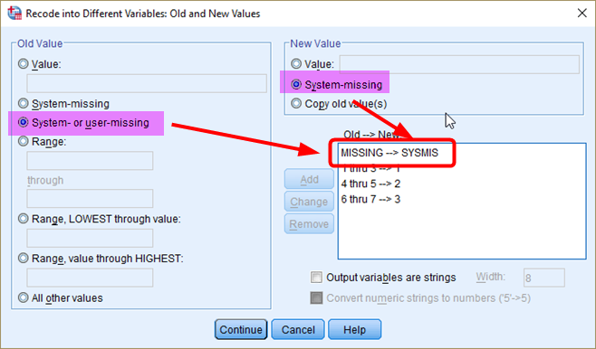
Figure 7: <Figure 7>
You already know this process. So I will not go into the details. However, I want to make sure that you should always provide the coding scheme for how missing values are treated. It is always best to choose the “System-” or “User- missing” (MISSING) to “System-missing” (SYSMIS)!!! In <Figure 6>, there is a category for 99 (No Answer). “No Answer” is assigned to 99, but this value is defined as missing values by users (Check the column of Missing). On the other hand, a system-missing happens when no information is available. “.” is used for showing system-missing (See <Figure 8>). If you do not include user-missing but include only system-missing in your recoding scheme (such as SYSMIS –> SYSMIS), then user-missing values such as 99 will be treated as valid categories (or values) in your newly recoded variable, which will ruin your subsequent analysis. In sum, always include “MISSING –> SYSMIS” when you recode variables.
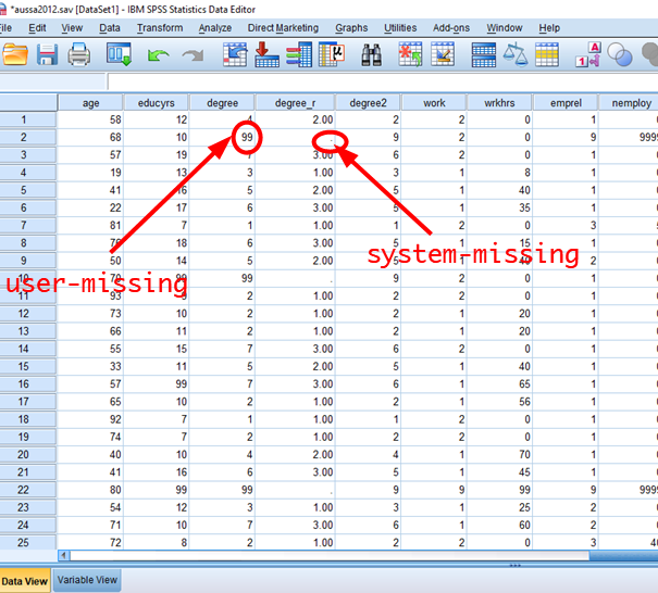
Figure 8: <Figure 8>
After recoding degree,recode age and topbot using the following recoding schemes. <Table 2> shows the recoding scheme for age, and <Table 3> for topbot.
| Values | Values | Labels |
|---|---|---|
| Lowest - 40 | 1 | 40 or less |
| 41 - 60 | 2 | 41 - 60 |
| 61 - Highest | 3 | 61 or more |
| Values | Values | Labels |
|---|---|---|
| 1 - 5 | 1 | Lower class |
| 6 - 8 | 2 | Middle class |
| 9 - 10 | 3 | Upper class |
Workshop Activity 9: Crosstabs and Chi-square |
|
1. Make a crosstab of newdegree (Education) and hubbywk (Attitudes toward traditional gender roles). Make sure that newdegree is an independent, and hubbywk is a dependent variable. Also, conduct a chi-square test of independence. Which statement describes best the relationship between education and the attitude toward traditional gender roles?
(1) More educated people are MORE likely to agree with traditional gender roles.
(2) More educated people are LESS likely to agree with traditional gender roles. (3) There is NO relationship between education and the attitude toward traditional gender roles. 2. Make a crosstab of newage (Age) and hubbywk (Attitudes toward traditional gender roles). Make sure that newage is an independent, and hubbywk is a dependent variable. Also, conduct a chi-square test of independence. Based on the chi-square test, what is your conclusion?
(1) Older people are MORE likely to agree with traditional gender roles. And this association is statistically significant at α =.05.
(2) Older people are MORE likely to agree with traditional gender roles. And this association is NOT statistically significant at α =.05. (3) Older people are LESS likely to agree with traditional gender roles. And this association is statistically significant at α =.05. (4) Older people are LESS likely to agree with traditional gender roles. And this association is NOT statistically significant at α =.05. (5) There is NO relationship between education and the attitude toward traditional gender roles. The association between them is NOT statistically significant at α =.05. 3. Make a crosstab of newtopbot (Class) and hubbywk (Attitudes toward traditional gender roles). Make sure that newtopbot is an independent, and hubbywk is a dependent variable. Also, conduct a chi-square test of independence. Based on the chi-square test, what is your conclusion?
(1) People from higher social classes are MORE likely to agree with traditional gender roles. And this association is statistically significant at α =.05.
(2) People from higher social classes are MORE likely to agree with traditional gender roles. And this association is NOT statistically significant at α =.05. (3) People from higher social classes are LESS likely to agree with traditional gender roles. And this association is statistically significant at α =.05. (4) People from higher social classes are LESS likely to agree with traditional gender roles. And this association is NOT statistically significant at α =.05. (5) There is NO relationship between social class and the attitude toward traditional gender roles. The association between them is NOT statistically significant at α =.05. |