0. Code to run to set up your computer.
# Update Packages
# update.packages(ask = FALSE, repos='https://cran.csiro.au/', dependencies = TRUE)

# Install Packages
if(!require(dplyr)) {install.packages("sjlabelled", repos='https://cran.csiro.au/', dependencies=TRUE)}
if(!require(sjlabelled)) {install.packages("sjlabelled", repos='https://cran.csiro.au/', dependencies=TRUE)}
if(!require(sjmisc)) {install.packages("sjmisc", repos='https://cran.csiro.au/', dependencies=TRUE)}
if(!require(sjstats)) {install.packages("sjstats", repos='https://cran.csiro.au/', dependencies=TRUE)}
if(!require(sjPlot)) {install.packages("sjlabelled", repos='https://cran.csiro.au/', dependencies=TRUE)}
if(!require(summarytools)) {install.packages("summarytools", repos='https://cran.csiro.au/', dependencies=TRUE)}
if(!require(ggplot2)) {install.packages("ggplot2", repos='https://cran.csiro.au/', dependencies= TRUE)}
if(!require(ggthemes)) {install.packages("ggthemes", repos='https://cran.csiro.au/', dependencies= TRUE)}
if (!require(GPArotation)) install.packages("GPArotation", repos='https://cran.csiro.au/', dependencies = TRUE)
if (!require(psych)) install.packages("psych", repos='https://cran.csiro.au/', dependencies = TRUE)
if (!require(ggrepel)) install.packages("ggrepel", repos='https://cran.csiro.au/', dependencies = TRUE)


# Load packages into memory
library(dplyr)
library(sjlabelled)
library(sjmisc)
library(sjstats)
library(sjPlot)
library(summarytools)
library(ggplot2)
library(ggthemes)
library(GPArotation)
library(psych)
library(ggrepel)

# Turn off scientific notation
options(digits=5, scipen=15)

# Stop View from overloading memory with a large datasets
RStudioView <- View
View <- function(x) {
  if ("data.frame" %in% class(x)) { RStudioView(x[1:500,]) } else { RStudioView(x) }
}

# Datasets
# Example 1: Crime Dataset
lga <- readRDS(url("https://methods101.com/data/nsw-lga-crime-clean.RDS"))
# extract just the crimes from crime dataset
first <- which( colnames(lga)=="astdomviol" )
last <- which(colnames(lga)=="transport")
crimes <- lga[, first:last ]

# Example 2: AuSSA Dataset
aus2012 <- readRDS(url("https://mqsociology.github.io/learn-r/soci832/aussa2012.RDS"))

# Example 3: Australian Electoral Survey
aes_full <- readRDS(gzcon(url("https://mqsociology.github.io/learn-r/soci832/aes_full.rds")))
# Codebook
browseURL("https://mqsociology.github.io/learn-r/soci832/aes_full_codebook.html")1. Theory: Dimension Reduction
1.1 What is a dimension?
We have learnt in earlier weeks that social science really happens in two separate, but interdependent realms: the realm of ideas - conceptualisation and theory - and the realm of experience - operationalisation, measurement, and empiricism.
Variables - characteristics of your units of analysis - exist at the conceptual and operational level.
But often, for a single theoretical concept - such as social class - ends up being measured by many different operationalisations in a dataset. In a survey, we might have questions about:
- Household income ($/year)
- Ownership of home (yes/no)
- Ownership of shares or property (yes/no)
- Occupation (high/medium/low status)
- Education (years of education)
If we did a correlation of these five variables, we would find - most likely - that they are highly correlated.
One of the ways of interpreting this correlation is that the five measures - the five operationalisations of wealth - are actually measuring the same single underlying conceptual variable - wealth.
We call this single underlying conceptual variable a ‘dimension’.
1.2 What is dimension reduction?
Dimension reduction is a set of analytical methods - factor analysis, multi-dimensional scaling, cluster analysis - which help identify underlying dimensions within a large correlated set of data.
We actually do a crude, qualitative, and intuitive form of dimension reduction everytime we divide people into categories in our mind and social conversations, such as when we make stereotypes, or make generalisations about ‘types’ or ‘groups’ of people.
In quantitative analysis, we use slightly more sophisticated methods to try to identify the underlying ‘dimensions’, ‘types’ or ‘clusters’ in our data. However, both the qualitative/intuitive, and quantitative methods of dimension reduction are based on the same underlying principle: we group together variables - characteristics - that correlate with each other and identify either (1) a smaller set of variables that capture most of the information contained the larger dataset, and/or (2) a set of groups of cases (people/individuals), who tend to have similar characteristics.
The exact mathematics behind these different methods of dimension reduction is beyond the scope of methods101.com (but it is briefly dealt with in the textbook and in the links to YouTube videos in the box below).
Key Terminology in Factor Analysis |
|
Factor: An unobserved (latent) variable that captures significant amounts of the variation of multiple observed variables. Factor loading: A measure of the correlation between an observed variable and the latent factor. Eigen decomposition (Spectral decomposition): A method of extracting factors from a correlation matrix. It works by reducing a correlation matrix of variables to a set of eigenvalues (integers), and eigenvectors (a row or column of numbers), which can be used to reconstruct the correlation matrix. These eigenvectors are the basis from which the factors are found, and the factor loadings calculated. Factor score: A number calculated from the factor loadings of a factor, and the values of the respective variables for an individual. It shows the score that this individual (case) has for this factor. For example, if we found their was a factor ‘wealth’, and we used the factor loadings of variables that are part of this factor, and the variables of an individual, we could work out a ‘wealth score’ (a factor score) for that individual. This ‘wealth score’ would indicate where this person sat on the wealth factor, relatively to other people in the dataset. |
But I really want to understand the underlying maths of Factor Analysis |
|
Below are six introductory videos of between 5 minutes and 20 minutes in length which explain as simply and as accurately as possible the underlying maths behind eigenvalues, eigevectors, and spectral decomposition. Calculating Eigenvalues and Eigenvectors 13 minute YouTube Video calculating Eigenvalues and Eigenvectors Explaining Eigenvalues and Eigenvectors Geometrically Eigen decomposition (spectral decomposition) Leah Howard, The Spectral Decomposition |
2. Steps in Factor Analysis
2.1 Step 1: Determine how many factors to extract.
Note that there are three main methods used in the literature:
- Number of factors whose eigenvalues > 1
- Number of factors whose eigenvalues are above the point of inflection
- Number of factors whose eigenvalues above simulated dataset with no factors
Generally method 3 is seen as best.
We can do this with the psych package function fa.parallel.
psych::fa.parallel(crimes,
  fm="pa",        # factor method to use (in this case I've used principle axis)
  fa="fa",        # eigen values for factor analysis (fa) shown, rather than principle componets
  use="pairwise"  # how to handle missing values (pairwise deletion)
  )
## Warning in cor.smooth(R): Matrix was not positive definite, smoothing was
## done## Warning in cor.smooth(r): Matrix was not positive definite, smoothing was
## done## Warning in fa.stats(r = r, f = f, phi = phi, n.obs = n.obs, np.obs
## = np.obs, : The estimated weights for the factor scores are probably
## incorrect. Try a different factor extraction method.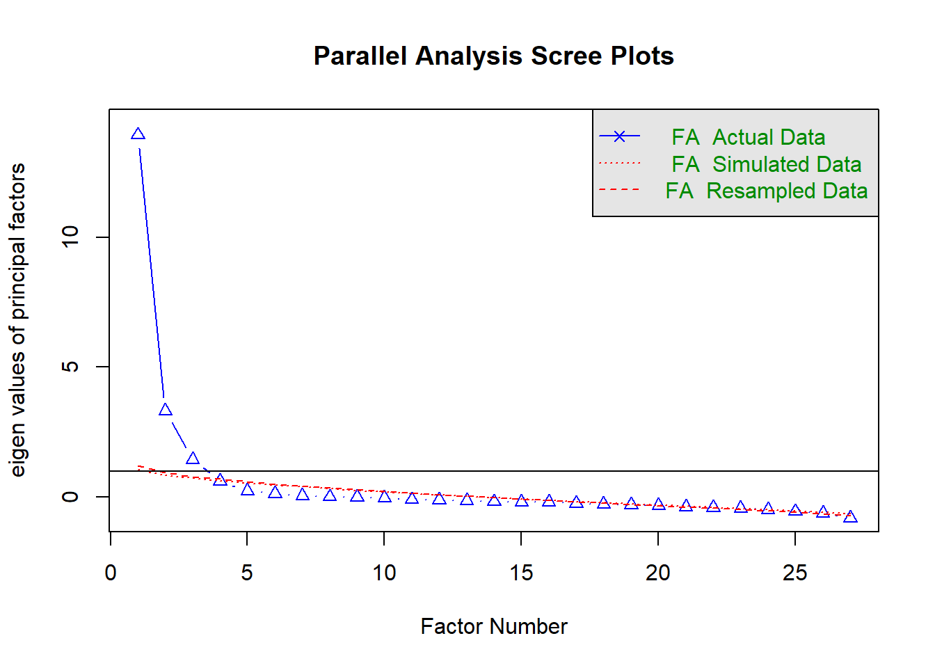
## Parallel analysis suggests that the number of factors = 3 and the number of components = NA2.2 Step 2: Choose factoring method and a rotation method
Factoring method: This is the algorithm used to find your factors. Each method uses different ways to try to find the ‘best’ factors that capture the most variance in your underlying dataset.
Some of the most common factoring methods used are:
- Maximum Likelihood “ml”
- Alpha “alpha”
- Ordinary Least Squares “ols”
- Minimum residual “minres”
- Principle axis factoring “pa”
It’s probably safest to use principle axis or maximum likelihood.
Rotation: Often the initial eigenvectors are difficult to interpret. Rotation is a method of keeping the information the same, but making it easier to interpret. You can think of it as being like keeping a pattern or shape the same, but turning it through X degrees rotation, until it ‘looks best’ and is easiest to interpret. Generally rotation tries to get all items to load on one factor only.
There are two main types of rotations:
orthogonal rotations: this is when the factors are kept at 90 degrees from one another - i.e. orthogonal - and so there is no correlation between the factors. Factors in an orthogonal rotation can be thought of as like the classic X and Y axis in a cartesian plot.
oblique rotations: this is when the factors are allowed to correlate with each other. Factors in an oblique rotation are more like two lines that cross, but cross at a 30 degree angle (for example).
Recommended rotations are:
ORTHOGONAL ROTATIONS
- “none”
- “varimax”
OBLIQUE ROTATIONS
- “promax”
- “oblimin”
results.1 <- psych::fa(r = crimes, nfactors = 3, rotate = "promax", fm="pa")## Warning in cor.smooth(R): Matrix was not positive definite, smoothing was
## done## Warning in fac(r = r, nfactors = nfactors, n.obs = n.obs, rotate =
## rotate, : A loading greater than abs(1) was detected. Examine the loadings
## carefully.## Warning in cor.smooth(r): Matrix was not positive definite, smoothing was
## done## Warning in fa.stats(r = r, f = f, phi = phi, n.obs = n.obs, np.obs
## = np.obs, : The estimated weights for the factor scores are probably
## incorrect. Try a different factor extraction method.results.1## Factor Analysis using method = pa
## Call: psych::fa(r = crimes, nfactors = 3, rotate = "promax", fm = "pa")
##
## Warning: A Heywood case was detected.
## Standardized loadings (pattern matrix) based upon correlation matrix
## PA1 PA3 PA2 h2 u2 com
## astdomviol 0.91 0.03 -0.06 0.85 0.154 1.0
## astnondomviol 0.58 0.38 0.19 0.87 0.133 2.0
## sexoff 0.56 0.33 -0.12 0.60 0.404 1.7
## robbery 0.54 0.08 0.48 0.71 0.291 2.0
## brkentdwel 1.01 -0.19 0.07 0.86 0.138 1.1
## brkentnondwel 0.85 -0.03 -0.08 0.66 0.338 1.0
## mottheft 0.95 -0.28 0.16 0.73 0.270 1.2
## steafrmot 0.87 -0.29 0.33 0.73 0.275 1.5
## steafrsto 0.19 0.07 0.74 0.70 0.296 1.2
## steafrdwel 0.78 0.13 -0.01 0.73 0.266 1.1
## steafrprsn -0.34 0.55 0.76 0.90 0.100 2.2
## fraud -0.14 0.03 0.90 0.78 0.222 1.0
## damtoprpty 0.96 0.00 0.01 0.93 0.074 1.0
## hrssthreat 0.86 0.09 -0.15 0.79 0.210 1.1
## recvstlgoods 0.29 0.16 0.70 0.80 0.201 1.5
## oththeft 0.11 0.58 0.44 0.79 0.208 1.9
## arson 0.91 -0.11 -0.03 0.71 0.290 1.0
## marijuana 0.09 0.61 0.11 0.50 0.501 1.1
## weapon 0.63 0.20 -0.20 0.54 0.460 1.4
## trespass 0.69 0.26 -0.18 0.71 0.292 1.4
## offcond 0.07 0.83 -0.03 0.75 0.248 1.0
## offlang 0.49 0.49 -0.21 0.70 0.296 2.3
## liqoff -0.33 0.93 0.16 0.69 0.311 1.3
## brchavo 0.89 0.03 -0.18 0.79 0.211 1.1
## brchbailcon 0.64 -0.03 0.30 0.57 0.433 1.4
## rsthindofficer 0.43 0.56 -0.02 0.77 0.227 1.9
## transport -0.17 -0.12 0.63 0.37 0.626 1.2
##
## PA1 PA3 PA2
## SS loadings 11.41 4.17 3.94
## Proportion Var 0.42 0.15 0.15
## Cumulative Var 0.42 0.58 0.72
## Proportion Explained 0.58 0.21 0.20
## Cumulative Proportion 0.58 0.80 1.00
##
## With factor correlations of
## PA1 PA3 PA2
## PA1 1.00 0.59 0.22
## PA3 0.59 1.00 0.29
## PA2 0.22 0.29 1.00
##
## Mean item complexity = 1.4
## Test of the hypothesis that 3 factors are sufficient.
##
## The degrees of freedom for the null model are 351 and the objective function was 75.38 with Chi Square of 8907.4
## The degrees of freedom for the model are 273 and the objective function was 47.25
##
## The root mean square of the residuals (RMSR) is 0.04
## The df corrected root mean square of the residuals is 0.05
##
## The harmonic number of observations is 111 with the empirical chi square 140.28 with prob < 1
## The total number of observations was 129 with Likelihood Chi Square = 5489.4 with prob < 0
##
## Tucker Lewis Index of factoring reliability = 0.202
## RMSEA index = 0.407 and the 90 % confidence intervals are 0.377 NA
## BIC = 4162.7
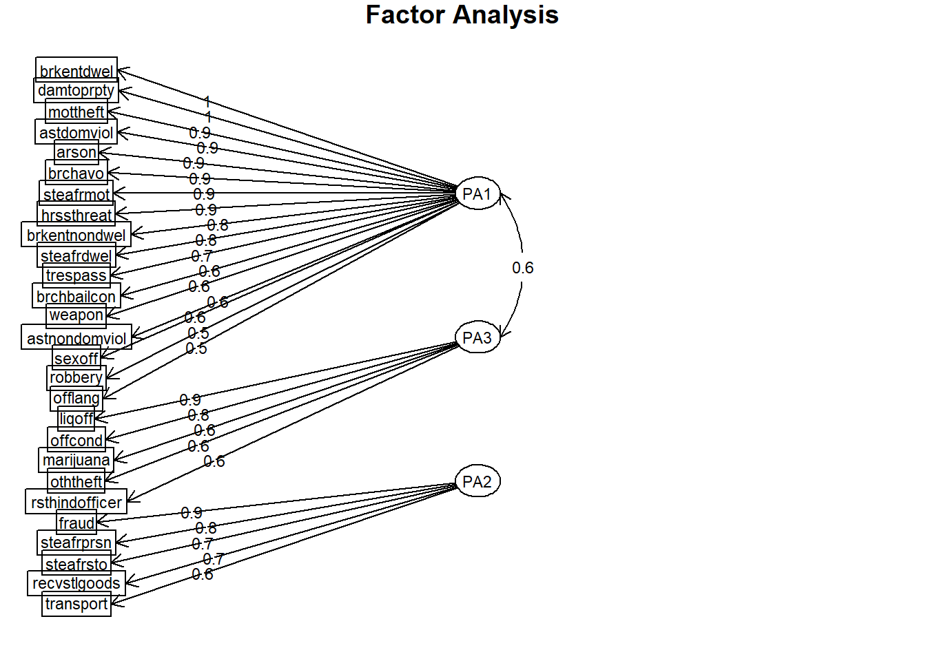
## Fit based upon off diagonal values = 0.992.3 Step 3: Visualise the factors
# (Step 4) Visualise the factors
psych::fa.diagram(results.1)