0. Code to run to set up your computer.
# Install Packages
if(!require(dplyr)) {install.packages("dplyr", repos='https://cran.csiro.au/', dependencies=TRUE)}
if(!require(sjlabelled)) {install.packages("sjlabelled", repos='https://cran.csiro.au/', dependencies=TRUE)}
if(!require(sjmisc)) {install.packages("sjmisc", repos='https://cran.csiro.au/', dependencies=TRUE)}
if(!require(sjstats)) {install.packages("sjstats", repos='https://cran.csiro.au/', dependencies=TRUE)}
if(!require(sjPlot)) {install.packages("sjPlot", repos='https://cran.csiro.au/', dependencies=TRUE)}

# Load packages into memory
library(dplyr)
library(sjlabelled)
library(sjmisc)
library(sjstats)
library(sjPlot)

# Turn off scientific notation
options(digits=3, scipen=8)

# Stop View from overloading memory with a large datasets
RStudioView <- View
View <- function(x) {
  if ("data.frame" %in% class(x)) { RStudioView(x[1:500,]) } else { RStudioView(x) }
}

# Datasets
# Example 5: Migrant Workers in Singapore
aw <- get(load(url("https://mqsociology.github.io/learn-r/soci832/aw.RData")))
1. Logistic regression
1.1 Example/Provocation
Open up the article using the link below:
Take a look at Table 2 on page 6 of the PDF. You can see five logistic regression models here.
Can you make sense of them?
See if you can answer these questions: 1. What is the dependent variable in each model? 2. What values can the dependent variable take? 3. What are the independent variables in each model? 4. What values can the independent variables take? 5. Why are there multiple models with the same dependent variable? 6. Why do we not include all independent variables in all the models? 7. How ‘good’ are each of the models? [Hint: R-square is an estimate of goodness of fit]
[note, if you are finding it hard to read the table in portrait, you can rotate the pages if you are in Adobe Acrobat by right clicking and choosing ‘rotate clockwise’]
1.2 R-code to reproduce these tables
# Model 1: SMI - simple model
model1 <- aw %>% glm(smi ~
               Age +
               Dependents +
               Salary +
               Hours +
               Construction +
               Bangladeshi +
               Uncleared_agent_fee,
               family="binomial", data = .)

summary(model1)
##
## Call:
## glm(formula = smi ~ Age + Dependents + Salary + Hours + Construction +
## Bangladeshi + Uncleared_agent_fee, family = "binomial", data = .)
##
## Deviance Residuals:
## Min 1Q Median 3Q Max
## -1.889 -0.975 -0.588 1.097 2.356
##
## Coefficients:
## Estimate Std. Error z value Pr(>|z|)
## (Intercept) -2.73515 0.75643 -3.62 0.00030 ***
## Age 0.02185 0.01841 1.19 0.23535
## Dependents 0.09258 0.11943 0.78 0.43822
## Salary -0.06450 0.02379 -2.71 0.00670 **
## Hours 0.02438 0.00674 3.62 0.00029 ***
## Construction -0.46067 0.18945 -2.43 0.01503 *
## Bangladeshi 1.05125 0.21355 4.92 0.00000085 ***
## Uncleared_agent_fee 0.72850 0.23611 3.09 0.00203 **
## ---
## Signif. codes: 0 '***' 0.001 '**' 0.01 '*' 0.05 '.' 0.1 ' ' 1
##
## (Dispersion parameter for binomial family taken to be 1)
##
## Null deviance: 781.90 on 581 degrees of freedom
## Residual deviance: 694.34 on 574 degrees of freedom
## AIC: 710.3
##
## Number of Fisher Scoring iterations: 3tab_model(model1)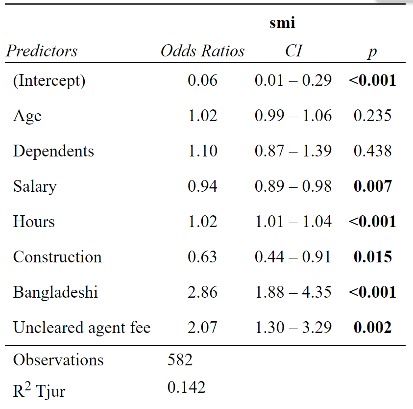
# Model 2 - Serious mental illness
model2 <- aw %>% glm(smi ~
              Age +
              Dependents +
              Salary +
              Hours +
              Construction +
              Bangladeshi +
              Ordinary_worker_x_Fee +
              Claimant_worker_x_Fee +
              Injury_dispute +
              Salary_dispute_only +
              Time_since_injury +
              Rent_empl +
              Threatened_with_deportation +
              Work_Permit +
              Threat_deport_x_Injury +
              Threat_deport_x_Salary,
              family="binomial", data = .)

summary(model2)
##
## Call:
## glm(formula = smi ~ Age + Dependents + Salary + Hours + Construction +
## Bangladeshi + Ordinary_worker_x_Fee + Claimant_worker_x_Fee +
## Injury_dispute + Salary_dispute_only + Time_since_injury +
## Rent_empl + Threatened_with_deportation + Work_Permit + Threat_deport_x_Injury +
## Threat_deport_x_Salary, family = "binomial", data = .)
##
## Deviance Residuals:
## Min 1Q Median 3Q Max
## -1.998 -0.847 -0.331 0.938 2.650
##
## Coefficients:
## Estimate Std. Error z value Pr(>|z|)
## (Intercept) -2.684374 0.893571 -3.00 0.0027 **
## Age 0.017307 0.020166 0.86 0.3908
## Dependents 0.013878 0.129948 0.11 0.9149
## Salary -0.029257 0.028859 -1.01 0.3107
## Hours 0.010244 0.007557 1.36 0.1752
## Construction -0.402165 0.208290 -1.93 0.0535 .
## Bangladeshi 0.773161 0.241855 3.20 0.0014 **
## Ordinary_worker_x_Fee 1.960191 0.688341 2.85 0.0044 **
## Claimant_worker_x_Fee 0.002408 0.261034 0.01 0.9926
## Injury_dispute 1.813572 0.438321 4.14 0.000035 ***
## Salary_dispute_only 1.605488 0.680152 2.36 0.0183 *
## Time_since_injury -0.000426 0.000696 -0.61 0.5408
## Rent_empl -0.714071 0.308823 -2.31 0.0208 *
## Threatened_with_deportation 1.839118 0.447170 4.11 0.000039 ***
## Work_Permit -0.132938 0.274211 -0.48 0.6278
## Threat_deport_x_Injury -1.515815 0.515509 -2.94 0.0033 **
## Threat_deport_x_Salary -0.467235 0.302691 -1.54 0.1227
## ---
## Signif. codes: 0 '***' 0.001 '**' 0.01 '*' 0.05 '.' 0.1 ' ' 1
##
## (Dispersion parameter for binomial family taken to be 1)
##
## Null deviance: 781.90 on 581 degrees of freedom
## Residual deviance: 596.77 on 565 degrees of freedom
## AIC: 630.8
##
## Number of Fisher Scoring iterations: 5tab_model(model2)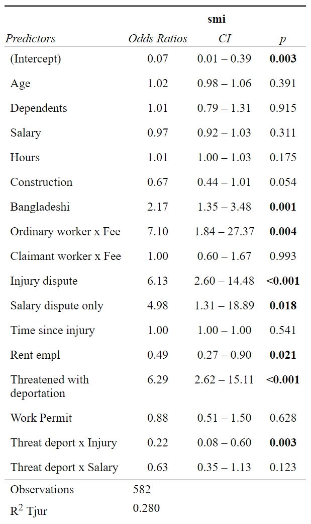
# Model 3 - Injury dispute
model3 <- aw %>% glm(Injury_dispute ~
               Age+Dependents +
               Salary +
               Hours +
               Construction +
               Bangladeshi +
               Uncleared_agent_fee,
               family="binomial", data = .)

summary(model3)
##
## Call:
## glm(formula = Injury_dispute ~ Age + Dependents + Salary + Hours +
## Construction + Bangladeshi + Uncleared_agent_fee, family = "binomial",
## data = .)
##
## Deviance Residuals:
## Min 1Q Median 3Q Max
## -2.613 -0.906 0.417 0.914 2.157
##
## Coefficients:
## Estimate Std. Error z value Pr(>|z|)
## (Intercept) -3.48717 0.81486 -4.28 0.0000187329 ***
## Age 0.03280 0.01978 1.66 0.097 .
## Dependents 0.25290 0.12803 1.98 0.048 *
## Salary -0.10666 0.02467 -4.32 0.0000154219 ***
## Hours 0.04037 0.00743 5.43 0.0000000559 ***
## Construction -0.25598 0.20418 -1.25 0.210
## Bangladeshi 1.24584 0.21064 5.91 0.0000000033 ***
## Uncleared_agent_fee 1.59031 0.30147 5.28 0.0000001326 ***
## ---
## Signif. codes: 0 '***' 0.001 '**' 0.01 '*' 0.05 '.' 0.1 ' ' 1
##
## (Dispersion parameter for binomial family taken to be 1)
##
## Null deviance: 801.03 on 581 degrees of freedom
## Residual deviance: 633.13 on 574 degrees of freedom
## AIC: 649.1
##
## Number of Fisher Scoring iterations: 4tab_model(model3)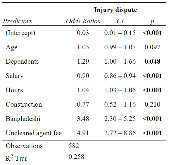
# Model 4 - Salary dispute
model4 <- aw %>% glm(Salary_dispute ~
                Age+Dependents +
                Salary +
                Hours +
                Construction +
                Bangladeshi +
                Uncleared_agent_fee,
                family="binomial", data = .)

summary(model4)
##
## Call:
## glm(formula = Salary_dispute ~ Age + Dependents + Salary + Hours +
## Construction + Bangladeshi + Uncleared_agent_fee, family = "binomial",
## data = .)
##
## Deviance Residuals:
## Min 1Q Median 3Q Max
## -1.256 -0.764 -0.652 -0.479 1.940
##
## Coefficients:
## Estimate Std. Error z value Pr(>|z|)
## (Intercept) -2.32773 0.80881 -2.88 0.0040 **
## Age 0.02907 0.01989 1.46 0.1439
## Dependents -0.04437 0.12898 -0.34 0.7309
## Salary -0.04765 0.02581 -1.85 0.0648 .
## Hours 0.00878 0.00715 1.23 0.2194
## Construction -0.10396 0.20595 -0.50 0.6137
## Bangladeshi 0.20198 0.22601 0.89 0.3715
## Uncleared_agent_fee 0.70633 0.23880 2.96 0.0031 **
## ---
## Signif. codes: 0 '***' 0.001 '**' 0.01 '*' 0.05 '.' 0.1 ' ' 1
##
## (Dispersion parameter for binomial family taken to be 1)
##
## Null deviance: 639.89 on 581 degrees of freedom
## Residual deviance: 619.55 on 574 degrees of freedom
## AIC: 635.5
##
## Number of Fisher Scoring iterations: 4tab_model(model4)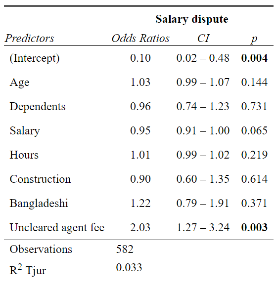
# Model 5 - Threat of Deportation
model5 <- aw %>% glm(Threatened_with_deportation ~
                Age +
                Dependents +
                Salary +
                Hours +
                Construction +
                Bangladeshi +
                Ordinary_worker_x_Fee +
                Claimant_worker_x_Fee +
                Injury_dispute +
                Salary_dispute_only,
                family="binomial", data = .)

summary(model5)
##
## Call:
## glm(formula = Threatened_with_deportation ~ Age + Dependents +
## Salary + Hours + Construction + Bangladeshi + Ordinary_worker_x_Fee +
## Claimant_worker_x_Fee + Injury_dispute + Salary_dispute_only,
## family = "binomial", data = .)
##
## Deviance Residuals:
## Min 1Q Median 3Q Max
## -1.631 -0.621 -0.423 0.965 2.353
##
## Coefficients:
## Estimate Std. Error z value Pr(>|z|)
## (Intercept) -2.39214 0.80933 -2.96 0.0031 **
## Age 0.00413 0.01971 0.21 0.8341
## Dependents -0.06985 0.12758 -0.55 0.5840
## Salary -0.04284 0.02815 -1.52 0.1280
## Hours 0.00999 0.00730 1.37 0.1710
## Construction -0.12787 0.20587 -0.62 0.5345
## Bangladeshi 0.31953 0.23399 1.37 0.1721
## Ordinary_worker_x_Fee 0.54652 0.81363 0.67 0.5018
## Claimant_worker_x_Fee 0.17676 0.25871 0.68 0.4945
## Injury_dispute 2.25203 0.25981 8.67 <2e-16 ***
## Salary_dispute_only 1.36508 0.61056 2.24 0.0254 *
## ---
## Signif. codes: 0 '***' 0.001 '**' 0.01 '*' 0.05 '.' 0.1 ' ' 1
##
## (Dispersion parameter for binomial family taken to be 1)
##
## Null deviance: 778.44 on 581 degrees of freedom
## Residual deviance: 613.24 on 571 degrees of freedom
## AIC: 635.2
##
## Number of Fisher Scoring iterations: 4tab_model(model5)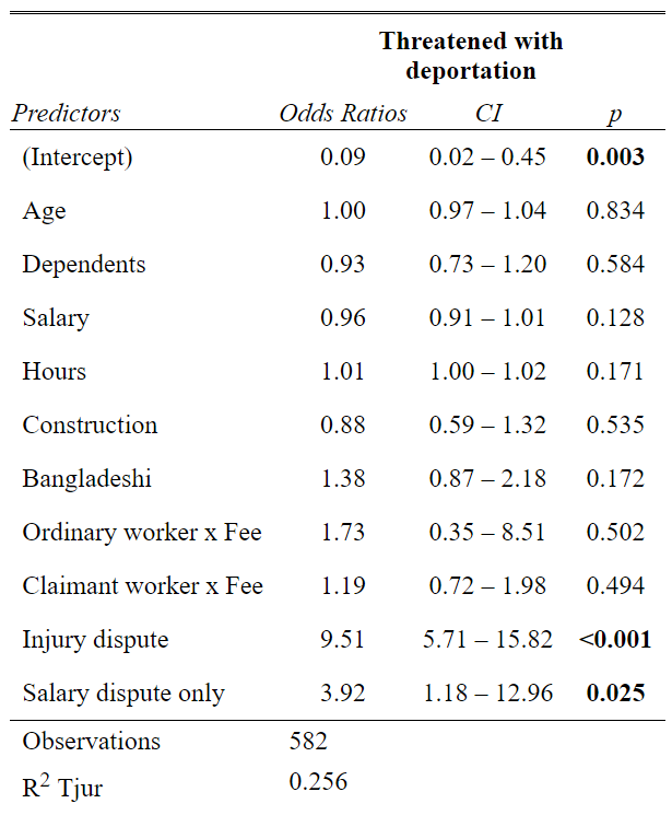
# Display as table
tab_model(model1, model2, model3, model4, model5, digits = 2,
          dv.labels = c("Model 1", "Model 2", "Model 3", "Model 4", "Model 5"),
          title = "Model of Serious Mental Illness in Migrant Workers in Singapore",
         show.se = FALSE, show.ci = FALSE)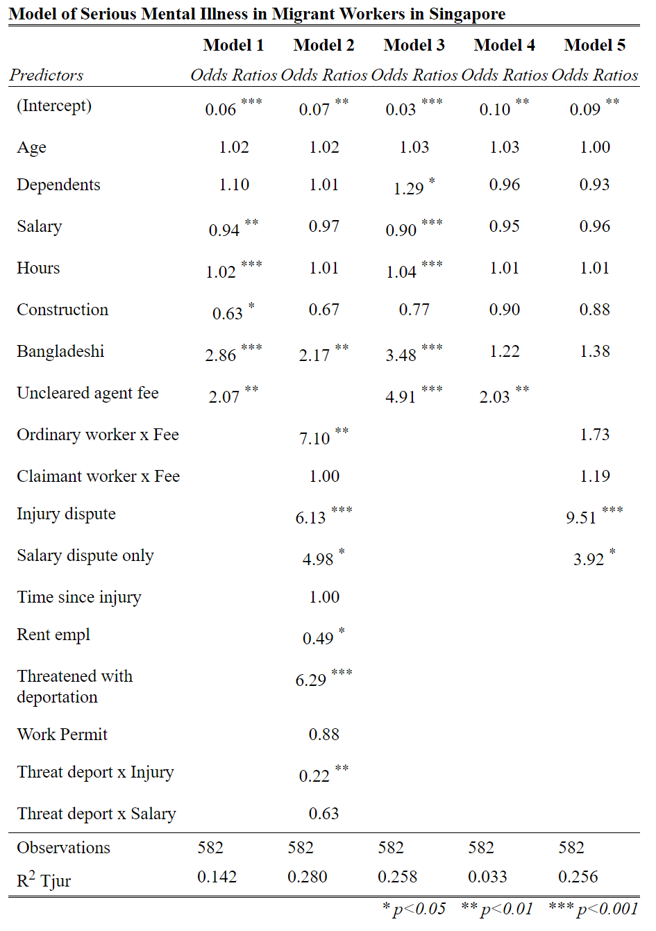
1.2 Summary of Logistic Regression
Some outcome variables are inherently binary:
- death
- catching a disease
- being cured
- pregnancy
- pass exam
- reelected to government
These are all inherently binary outcomes.
Such outcomes violate many of the basic assumptions of linear regression models, and so we can’t use them.
For example, what would it mean that drinking a glass of red wine each night reduced your chance of dying by 0.1 units of death?
It doesn’t make sense.
To deal with this inherent limitation of linear regression models, statistians developed the logistic regression (or logit) model, and also a related model called probit.
Like a linear regression model, a logistic regression model uses a linear model of the relationship between the predictor (independent) variables, and the outcome (dependent) variable.
What logisitic regression models change is the link - the function - by which one unit of predictor influences the outcome.
Whereas the equation for linear regression is:
\[y = Bx + c\]
The equation for a similar logit is:
\[\text{Probability}(y=1) = \frac{1}{\left(1+e^{-(Bx+c)}\right)}\] \[\text{Where:}\] \[e = \text{ base of natural log (approximately 3)}\]
If that equation looks confusing to you DON’T WORRY, because it is!!!
The reason the equation is confusing is because really it makes more sense if we write it as this.
\[\text{log}\left(\frac{y}{(1-y)}\right) = Bx + C\]
or even more simply
\[\text{logit}(y) = Bx + C\]
The best explanation for this is on this statistics webpage for UCLA https://stats.idre.ucla.edu/other/mult-pkg/faq/general/faq-how-do-i-interpret-odds-ratios-in-logistic-regression/
I will, however, try to summarise what it says.
Even though we have a binary outcome we do still want to be able to say something like “for each unit increase in X (e.g. glasses of wine) there is B unit increase in the probability of Y (e.g. dying in a car crash when you drive home).”
Thus, the right hand side of the equation (Bx + C) remains the same.
On the left side of the equation, which is ‘y’ in a linear regression, we would - as humans who think in simple terms - ideally like ‘y’ to be a probability of an event.
It turns out - when we consult our mathematical friends - there are at least two major problems with just making ‘y’ a probability:
- First: Outcome should not have bounds. Probabilities range from zero to one, and when you are estimating a mathematical equation, it is difficult to have a variable that is bound between two values (0 and 1)
- Second: Outcome variable values should increase linearly across whole range of values Unit increments of probability (from 0.5 to 0.59999, or 0.9 to 0.99999) are not linear. In the above two examples, a 0.09999 change in probibility shifts means much more when it increases an event from 9 in 10 (90% certainty) to almost 100% certainty, than it does when it simply changes the chance of something happening from 50:50 to 6/10.
- Our mathematical friends, however, have found a solution, which is to undertake two transformations of a probability, to make it into a number that is ‘well behaved’ and doesn’t suffer from these problems of limited range, and non-linearity. The two transformations are:
- First: TRANSFORM PROBABILTY TO ODDS. Odds are (p/(1-p)), which means: the chance of something happening (p), divided by the chance of it not happening (1-p). This number still has the problem of only having a range of 0 to positive infinity. And also it is non-linear (compare moving from 0 to 1 and from 1 to 2, or 1 to infinity),
- Second: TAKE THE LOG OF THE ODDS. This solves both problems, providing a variable with range from minus infinity to plus infinity, and which has a distribution around the probability of 0.5 which is ‘similar’ to a normal distribution.
- A key thing to notice here is that the ‘form’ of a logistic regression is very similar to that of a linear regression. The right hand side (the predictor variables) is the same, while the left hand side, we still have ‘y’ - the dependent variable -, but we have transformed it by taking the log-odds.
If you look again at the two equations, they should look a little less scary now.
\[\text{logit}(y) = Bx + C\]
\[\text{log}\left(\frac{y}{(1-y)}\right) = Bx + C\]
- Remember that when we report regression coefficients, we are reporting estimated values for ‘B’ in the above equations.
It turns out that when we report ‘B’ in regression models we report it measured in one of two units:
- LOG-ODDS (Range minus infinity to plus infinity; no effect is log-odds = 0): coefficients are generally output in most statistical packages as ‘log-odds’. Generally we just called these ‘coefficients’. Note that they vary from minus infinity to plus infinity, and ‘no effect’ is when the coefficient is zero. This coefficient is often called ‘B’.
- ODDS RATIO (Range 0 to plus infinity; no effect is odds ratio = 1): when actually discussing our results and when publishing regression tables in journals, we generally transform our coefficients into ‘odds ratios’, which is simply the exponential of B. Remember the basic mathematical rule which is that the natural log and exponential are inverse operations, so exp(log(p/(1-p))) = p/(1-p) The exp and log just cancel each other out. These cofficients are often called ‘Exp B’ or ‘Odds Ratio’.
1.3 Another good example from UCLA
https://stats.idre.ucla.edu/r/dae/logit-regression/