Creating a Dataset of Complete Cases

In most cases, your dataset contains cases with many missing values. Missing values can reduce the statistical power of analyses and produce biased estimates, which could lead to invalid conclusions. There are several ways to handle missing values, but this lab introduces only the listwise deletion (also known as complete-case analysis) which is the most frequently used method in handling missing data. Listwise deletion removes any case in a dataset if the case has a missing value on any variable in the analysis. Suppose that we are investigating the relationships across six variables: sexual offence rates (sexoff), the median age of residents (medage), unemployment rates (unemploy), median house prices (housmedprice), regions of LGAs(region2), and urban or rural LGAs (urban). The first step of this analysis is to create a dataset which includes only LGAs that have no missing values on these six variables so that we can investigate all the relationships based on the same set of LGAs. First, we create a new dataset (crime2) which has the six variables of our choice as well as identification numbers (code) and LGA names (name). Note that code and name have no missing values and thus does not affect the listwise deletion process. select() is used for choosing variables that will be included in a new dataset. If you are not familiar with this function, go to Creating a dataset of specific variables.

crime2 <- crime %>%
  select(code, name, medage, unemploy, housmedprice, sexoff, region2, urban)

Second, we make a new variable (mark), which will show whether cases have missing values on any of the six variables. We tentatively assign 0 to all the cases. ‘mutate()’ is used for creating a new variable. If you are not familiar with this function, go to Computing variables.

crime2 <- crime2 %>%
  mutate(mark = 0)

Third, we replace 0 with 1 only when cases do not have missing values on all the six variables. Thus, 1 indicates cases with no missing values, and 0 indicates those with missing values. ‘replace(variable, condition, value)’ will change the value of variable into value when condition is met. ‘complete.cases(data)’ identifies cases with no missing values in data. Taken together, the code assigns 1 to cases only when they have no missing values.

crime2 <- crime2 %>%
  mutate(mark = replace(mark, complete.cases(crime2), 1))

Finally, we keep only cases with no missing values. ‘filter()’ is used for selecting complete cases. If you are not familiar with this function, go to Creating a dataset of a sub-group.

crime2 <- crime2 %>%
  filter(mark == 1)

We will use this newly created dataset in the remaining analyses.

Changing the Scale of Variables

housmedprice has a huge range (47,500 – 2,800,000), which makes it a little bit difficult to interpret regression outputs. Therefore, reducing the range would be helpful. An easy way to achieve this goal is to divide the value by numbers. In this example, we divide it by 10,000. The following code performs this task and assigns a new variable label.

crime2 <- crime2 %>%
  mutate(housmedprice = housmedprice/10000)
crime2$housmedprice <- set_label(crime2$housmedprice, label = "Median sale price of house ($10,000)")

Computing and Visualising Correlation Coefficients

Let’s examine the relationship between two continuous variables, median house prices (housmedprice) and sexual offence rates (sexoff). To compute correlation coefficients of two continuous variables, use cor(data$variable1, data$variable2, method = “pearson”, use = “complete.obs”). This shows a Pearson correlation coefficient based on complete cases (which has no missing values on two variables of your choice). The following codes compute the correlation coefficient between housmedprice and sexoff.

cor(crime2$sexoff, crime2$housmedprice, method = "pearson", use = "complete.obs") 

## [1] -0.52149

The output shows that the correlation coefficient is -0.52149.

We visualise the relationship using plot_scatter(data, independent, dependent). We assume that median house prices influence sexual offence rates. Thus, housmedprice is an independent, and sexoff is a dependent variable. Thus, the following code shows a scatterplot between housmedprice and sexoff.

plot_scatter(crime2, housmedprice, sexoff, colors = "#8B1A1A88", dot.size = 3, fit.line = "lm")

## `geom_smooth()` using formula 'y ~ x'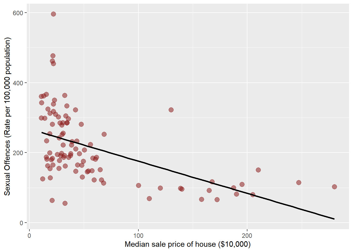

Note that ‘colors’ assign the colour of dots (I assigned a transparent colour in the above code so that we can easily notice overlapped dots), ‘dot.size’ set the size of dots, and ‘fit.line = “lm”’ adds a linear fitted line to the scatterplot.

Producing a Correlation Matrix

‘cor()’ allows us to compute a correlation coefficient between only two variables. But what if we want to calculate correlation coefficients across many variables of our choice simultaneously? The correlation matrix could be an easy solution. It is a way of presenting multiple correlation coefficients in a single table. Variables are arrayed across the left (in the first column) and across the bottom (in the last row). Correlation coefficients for each relationship appear in the corresponding cell of the table.

To produce a correlation matrix, we need to create a new dataset (corr.crime) consisting of variables across which correlation coefficients are computed. In the following example, we calculated them across four variables: medage, unemploy, housmedprice, sexoff. Therefore, we select these variables from the complete-case dataset we made (crime2).

corr.crime <- crime2 %>%
  select(medage, unemploy, housmedprice, sexoff)

Let’s check which variables are included in corr.crime.

names(corr.crime) 

## [1] "medage"       "unemploy"     "housmedprice" "sexoff"

The output confirms that the variables we selected are included. It also shows the order of variables: medage is in the leftmost column, and sexoff is in the rightmost column. Next, we will change this order so that we can read correlation coefficients easily. sexoff (4th) should come first, then unemploy (2nd), then housmedprice (3rd), and finally medage (1st). The following code performs this task. c(4, 2, 3, 1) tells R this new order.

corr.crime <- corr.crime[,c(4,2,3,1)] 

Now, let’s make a correlation matrix using sjp.corr(data).

sjp.corr(corr.crime)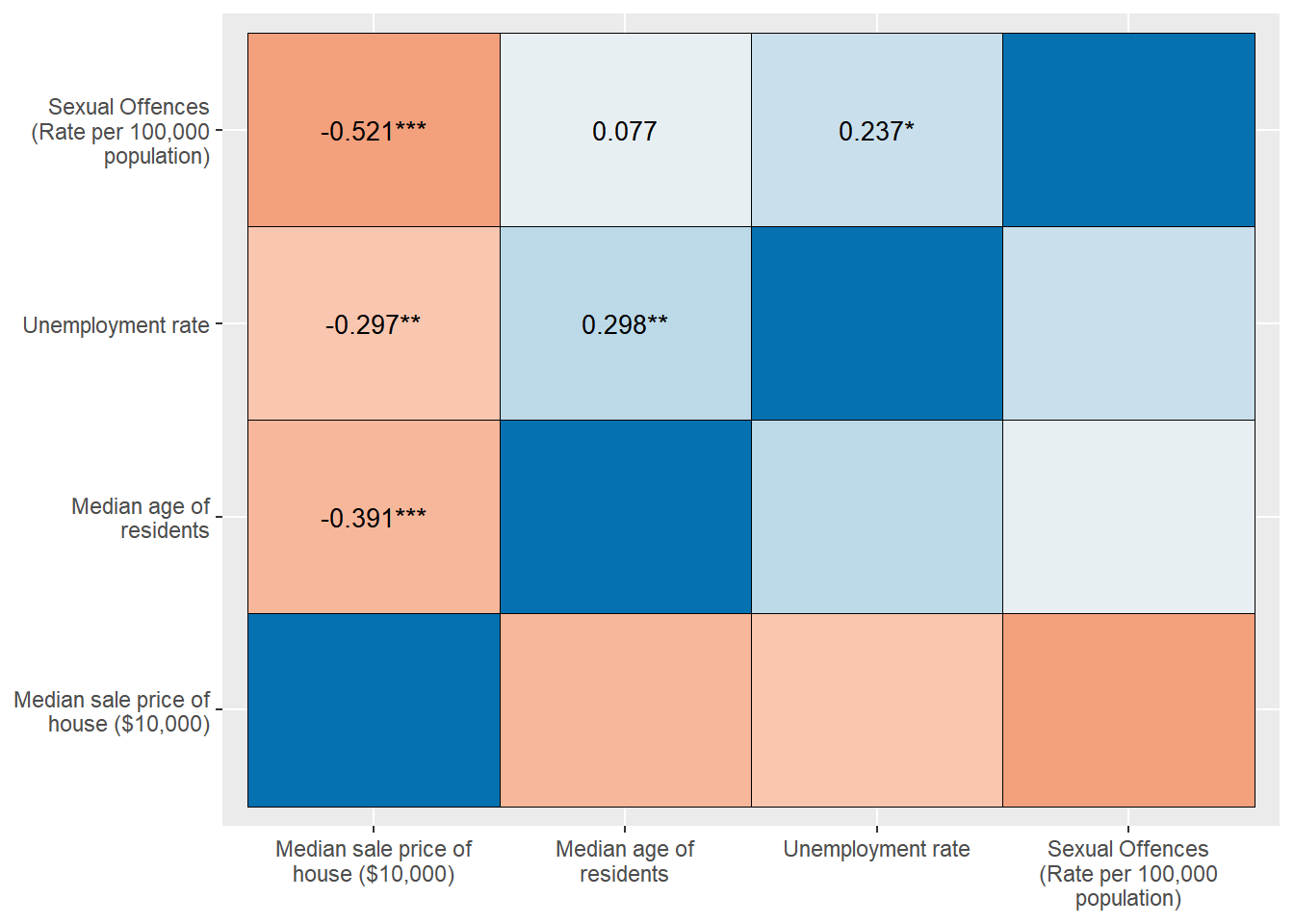

The output shows all the coefficients across the four variables of our choice. Also, colours tell the coefficient indirectly. Red colours indicate negative, and blue colours suggest positive correlations. The darker a colour is, the stronger the relationship is.

Simple Regression Analysis

Regression analysis is a more advanced way to examine the relationship between two variables. Let’s examine the relationship between median house prices (housmedprice) and sexual offence rates (sexoff) again using a regression model. lm(dependent ~ independent, data = data name) is used for computing regression coefficients. Also, you need to assign a model name using model name <-. In the following code, we assign a model name as model.1.

model.1 <- lm(sexoff ~ housmedprice, data = crime2)

After running this code, you do not see any R output. To see regression outputs, run summary(model name). It will show the output.

summary(model.1)

## 
## Call:
## lm(formula = sexoff ~ housmedprice, data = crime2)
## 
## Residuals:
##    Min     1Q Median     3Q    Max 
## -184.6  -61.3  -17.5   55.5  348.4 
## 
## Coefficients:
##              Estimate Std. Error t value             Pr(>|t|)    
## (Intercept)   267.818     12.446   21.52 < 0.0000000000000002 ***
## housmedprice   -0.919      0.154   -5.99          0.000000037 ***
## ---
## Signif. codes:  0 '***' 0.001 '**' 0.01 '*' 0.05 '.' 0.1 ' ' 1
## 
## Residual standard error: 87.6 on 96 degrees of freedom
## Multiple R-squared:  0.272,  Adjusted R-squared:  0.264 
## F-statistic: 35.9 on 1 and 96 DF,  p-value: 0.0000000367

In the output, the intercept is 267.818, which means that sexual offence rates will be 267.8 if the median sale price of houses is $0. The coefficient of housmedprice is -0.919, which means that for each additional $10,000 in the median sale price of houses, sexual offence rates will decrease by 0.919. This negative effect of housmedprice is statistically significant at α = .05 because the p-value (0.000000037) is much less than .05. The regression equation of this model is \(sexoff = -.919 × housmedprice + 267.8\). The coefficient of determination (Multiple R-squared) is 0.272, which means that 27.2% of the total variance in sexual offence rates is explained by the median house price.

The R codes you have written so far look like:

################################################################################
# Lab 10: Correlations & Simple Regression
# 24/05/2021
# SOCI8015 & SOCX8015
################################################################################

# Load packages
library(dplyr)
library(sjlabelled)
library(sjmisc)
library(sjPlot)

# Avoid scientific notation
options(digits=5, scipen=15) 

# Load datasets
crime <- readRDS("nsw-lga-crime.RDS")

# Creating a Dataset of Complete Cases
crime2 <- crime %>%
  select(code, name, medage, unemploy, housmedprice, sexoff, region2, urban)

crime2 <- crime2 %>%
  mutate(mark = 0)

crime2 <- crime2 %>%
  mutate(mark = replace(mark, complete.cases(crime2), 1))

crime2 <- crime2 %>%
  filter(mark == 1)

# Changing the Scale of Variables
crime2 <- crime2 %>%
  mutate(housmedprice = housmedprice/10000)
crime2$housmedprice <- set_label(crime2$housmedprice, label = "Median sale price of house ($10,000)")

# Computing and Visualising Correlation Coefficients
cor(crime2$sexoff, crime2$housmedprice, method = "pearson", use = "complete.obs") 
plot_scatter(crime2, housmedprice, sexoff, colors = "#8B1A1A88", dot.size = 3, fit.line = "lm")

# Producing a Correlation Matrix
corr.crime <- crime2 %>%
  select(medage, unemploy, housmedprice, sexoff)
names(corr.crime) 
corr.crime <- corr.crime[,c(4,2,3,1)] 
sjp.corr(corr.crime)

# Simple Regression Analysis
model.1 <- lm(sexoff ~ housmedprice, data = crime2)
summary(model.1)