====================================
Reading |
|
Field, A., Miles, J., and Field, Z. (2012). Discovering statistics using R. Sage publications.
|
Concepts |
Overview: Intro to R and R Studio |
|
Questions
Exercises
|
====================================
Reading |
|
Field, A., Miles, J., and Field, Z. (2012). Discovering statistics using R. Sage publications.
|
Concepts |
Overview: Intro to R and R Studio |
|
Questions
Exercises
|
A lot of the most basic statistical analysis can be done in Microsoft Excel, and for very simple things this will be your best option.
Another very popular statistical package is SPSS by IBM. This package has the advantage of having a Graphical User Interface (GUI), which means you can run most commands by pointing and clicking with a mouse.
However, for this course we are using R. Why R? There are three main reasons.
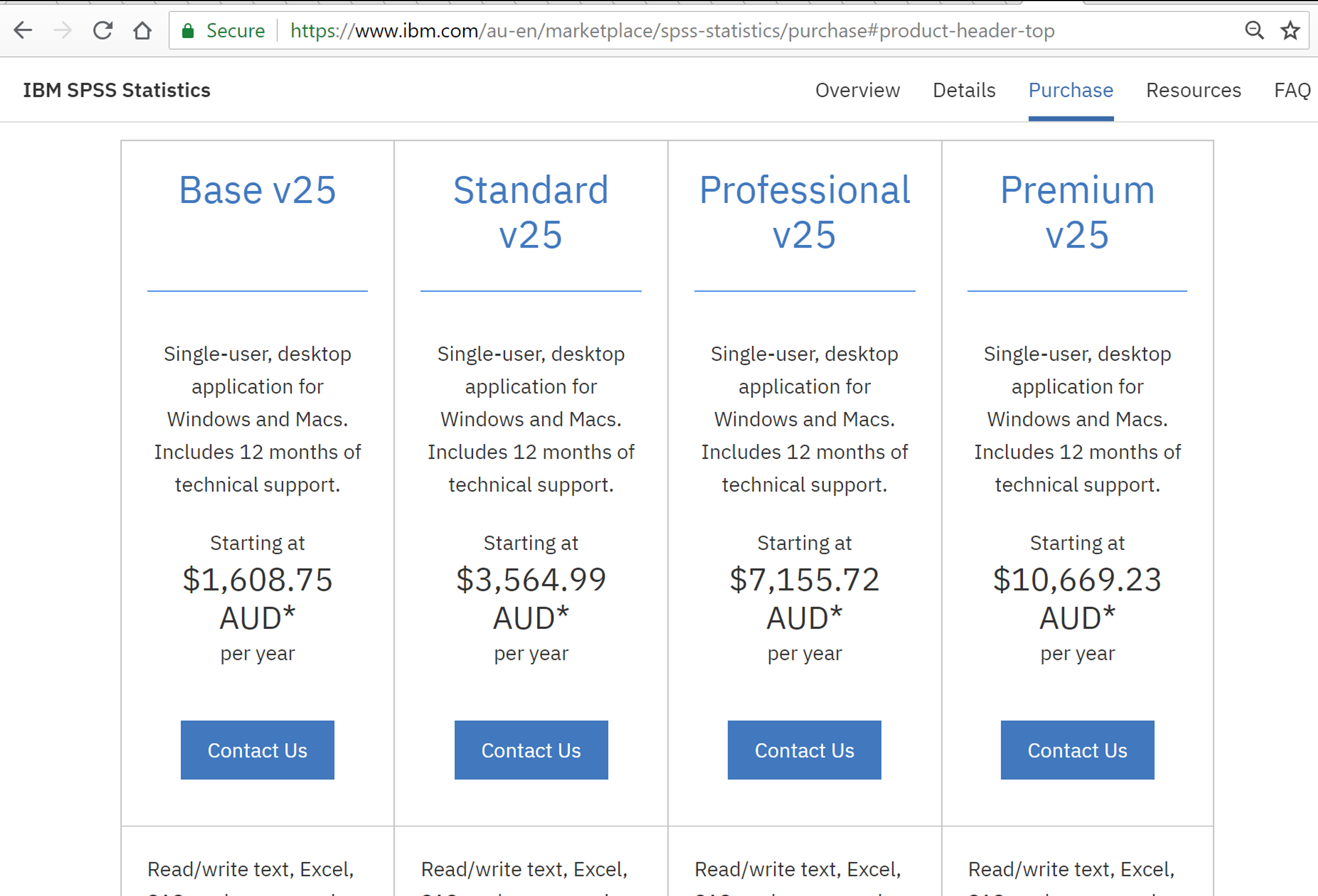
Figure 1: Cost of SPSS licences per year (26/7/2018).
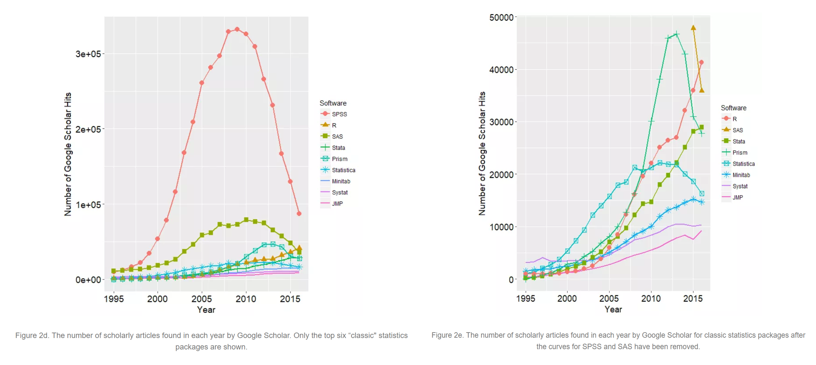
Figure 2: Scholarly articles using each major statistical package.
Source: http://r4stats.com/articles/popularity/
Installing & Updating R and R Studio |
|
I have written a detailed walk through of the steps to install R and RStudio here: Appendix 1: Installing R and RStudio. Updating R and R StudioIt is generally a very good idea - particularly when working along with instructions in this class - to make sure you are using the latest versions of R Studio and R. If you installed either more than a month ago, then chances are they our out of date. However, you can just check by following these instructions
In RStudio:
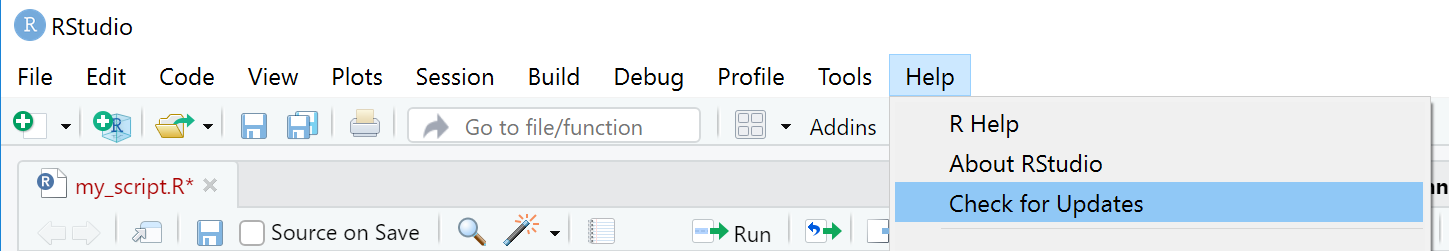
Figure 3: How to check your RStudio version is current. 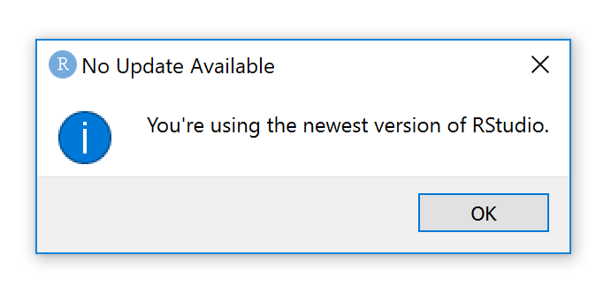
Figure 4: How to check your RStudio version is current.
What version of R am I using? You can tell which version of R you are running by looking in RStudio, in the Console window, as you can see in Figure 5. 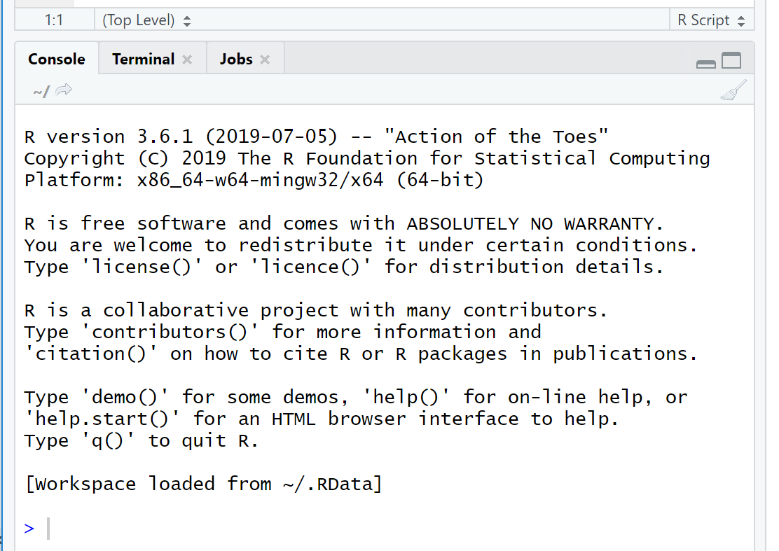
Figure 5: How to check your RStudio version is current. What is the latest version of R? In any browser:
You can see the version number on this page. If you are not uptodate, then on the pages above simply:
Once the new version of R is installed need to close RStudio, and then reopen it. RStudio should automatically recognise the new version of R. You can confirm the new version of R is installed by lookibng at the version number of R in the console window (as explained just above in Figure 5). |
COMMON CONFUSION: We almost never open R directly. We just open RStudio. |
|
One common mistakes people new to R and RStudio make is to think that they need to directly open R on their computer. You don’t. You don’t need to click on the R icon and open it at any stage. Instead, we just open RStudio, and RStudio will communicate with R for us. RStudio is a nice interface that makes it much easier to use R. |
When you first open RStudio you should see something like Figure 6.
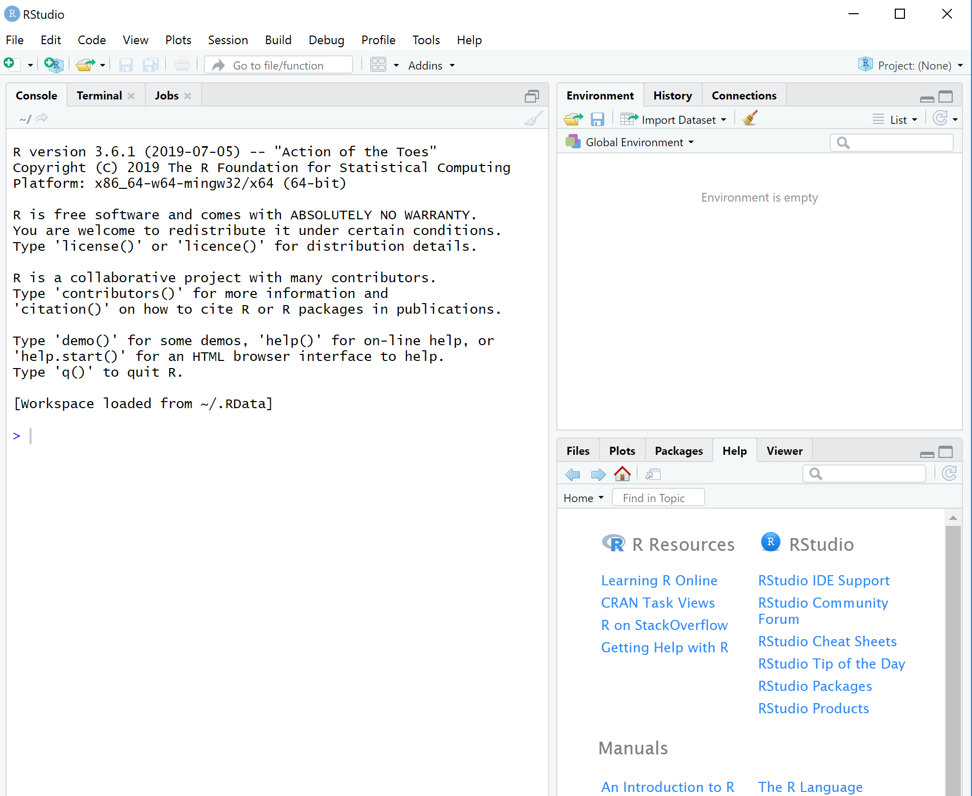
Figure 6: What RStudio looks like when we first open it.
The first thing you want to do is open a new project.
A project is like a separate workspace you create for each of your areas of work, such as your thesis, or an assignment, or a project at work. Each project will have its own working director, files, folders, and history.
Step 1: To open a project go to File and then New Project, as shown in Figure 7.
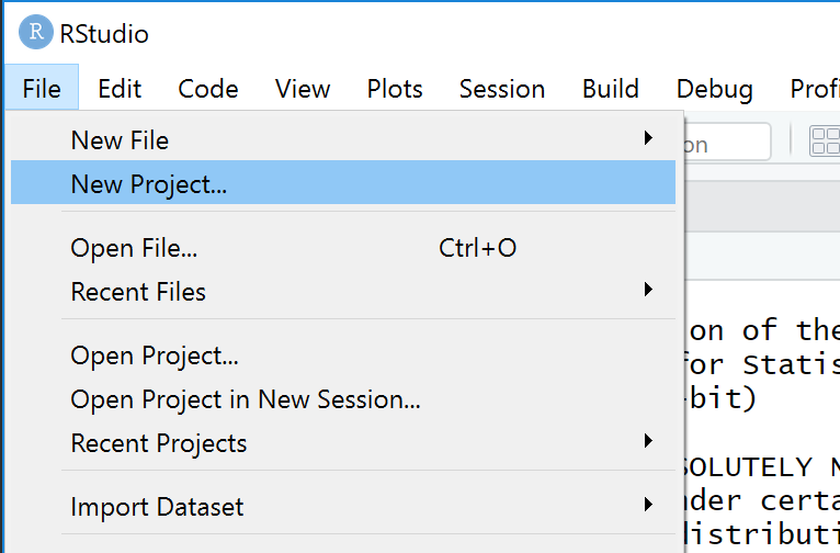
Figure 7: Step 1: How to open a new project in RStudio.
Step 2: In the window that opens, you have a number of choices. At this stage, select “New Director”, as shown in Figure 8.
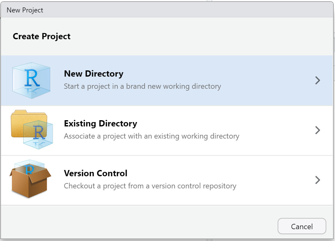
Figure 8: Step 2: How to open a new project in RStudio.
Step 3: Select “New Project”, as shown in Figure 9.
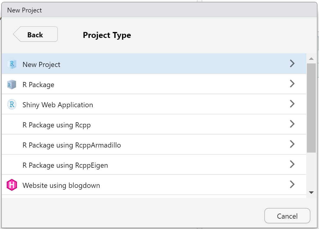
Figure 9: Step 3: How to open a new project in RStudio.
Step 4: Type in the name of your new directory. In my case I am creating one called “2019, SOCI832 Practice” Figure 10.
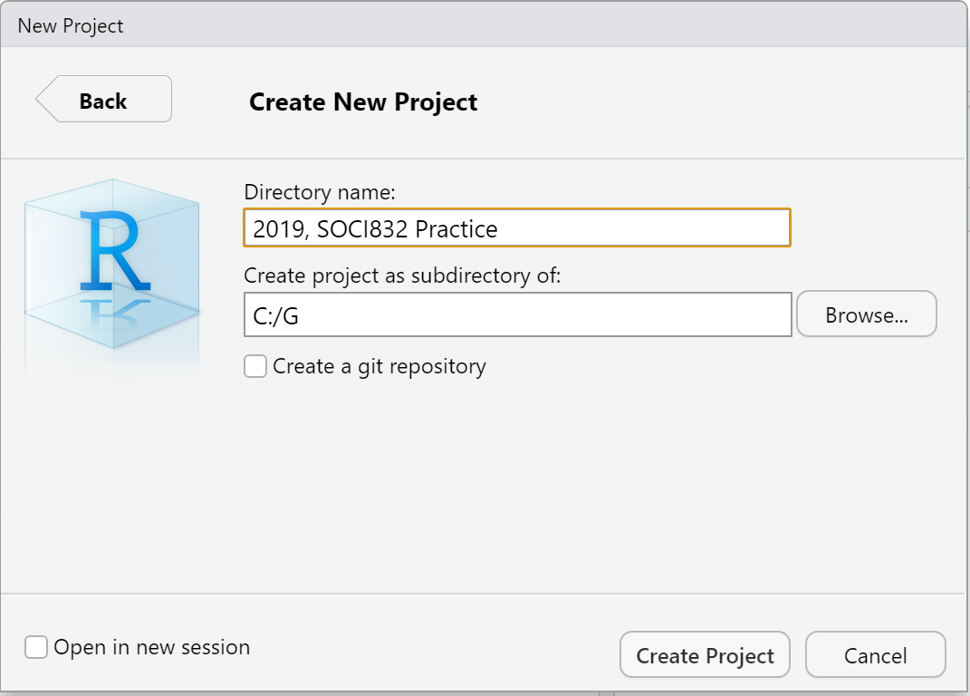
Figure 10: Step 4: How to open a new project in RStudio.
Step 5: RStudio will now open a new project for you. You can see the name of the folder at the top of the RStudio window, and also under the ‘Console’ tab.
The next thing we want to do, before we really get started with RStudio, is open a script file.
As you probably know, we need to type commands into R - we can’t just point and click like we do in Microsoft Word or SPSS.
When we type commands, two things happen:
Using a script - which is basically just a text file with all our commands in it - allows us to correct our mistakes, save our commands, and also copy and paste them later when we want to do similar analysis.
Step 1: To open a script file go to File menu and then New File and then R Script as shown in Figure 11.
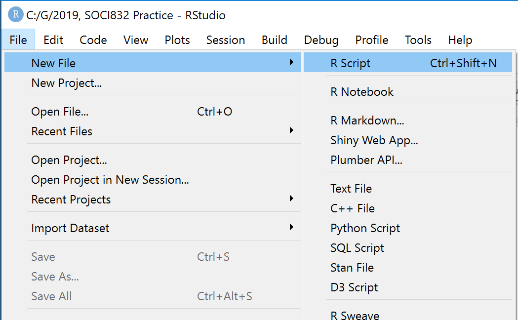
Figure 11: Step 4: How to open a new script file in RStudio.
There are also two short cuts to doing this:
Step 2: To save your script file go to the menu File and then Save As. Navigate to your folder (in my case C:019, SOCI832 Practice), and then give your script file a name. I will call mine nicks_script. And press Save
Let’s run your first script.
In the script window you can type the classic first command of any book that teaches programming.
print("Hello World")And then put your cursor anywhere on that line of code in the script window and press Ctrl+Enter (in Windows) or Cmd+Enter (on a Mac).
In the console window (below the script) you should see this.
## [1] "Hello World"Actually, what you will see in the console window is what appears in Figure 12.
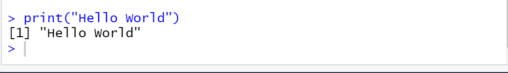
Figure 12: Output in Console window from print("Hello World") command.
What does it mean?
It is a command that says “Print to the console the text inside the double inverted commas”, which in our case is “Hello World”.
It is a pretty useless command, but it shows how you can run a line in a script file, and see the results in the console window.
Lets take a quick look around RStudio, and orient ourselves.
Figure 13 shows what RStudio looks like in a default setting.
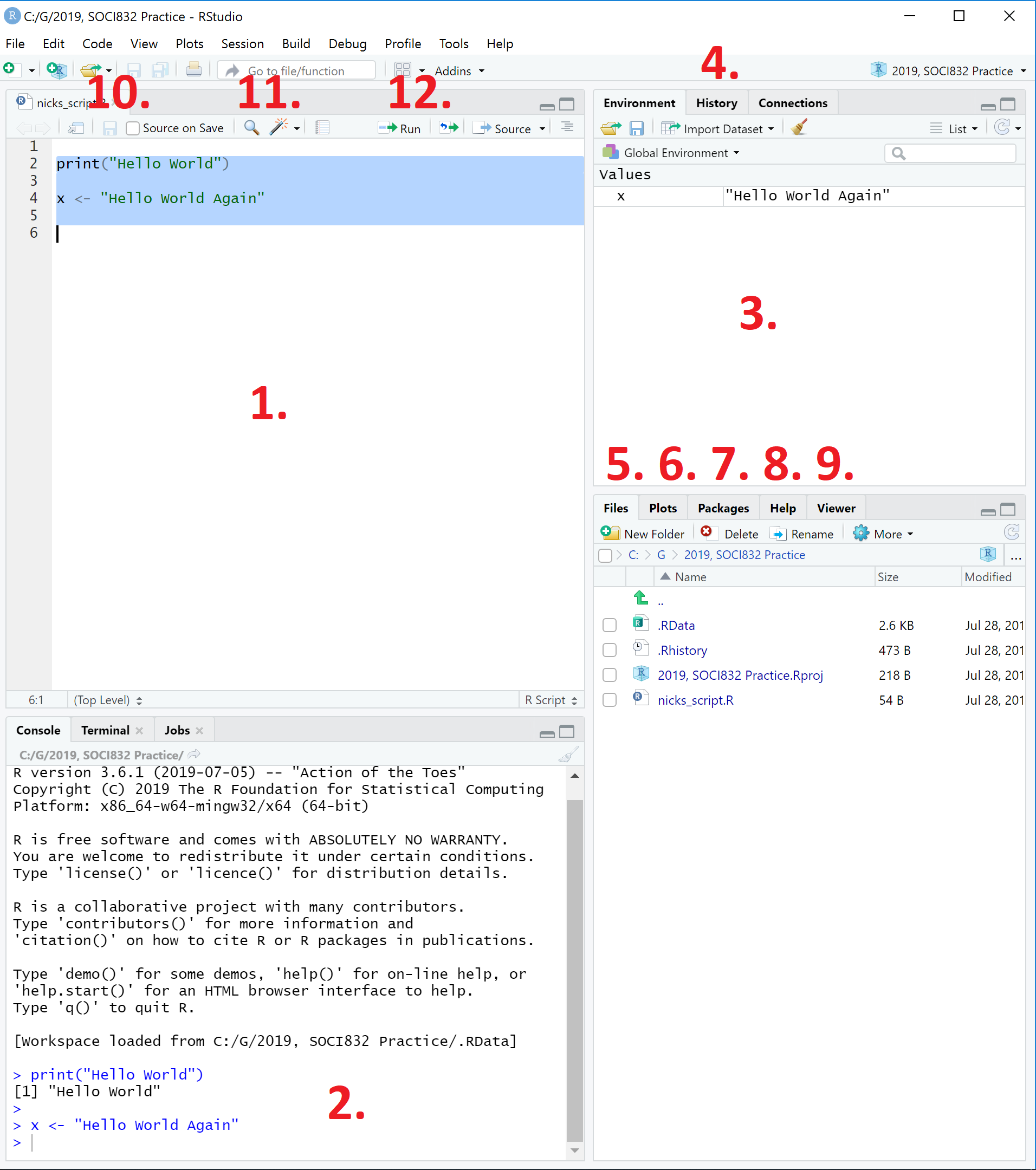
Figure 13: Looking around the RStudio interface.
The numbers in Figure 13 refer to:
In this section we are going to learn about (1) simple objects in R (often called variables in other programming languages); (2) conducting calculations on these objects; and then (3) transforming these objects with functions.
We can create a simple object with this command:
x <- "Hello World"In R we call <- the assignment operator. It says “Put the value on the right into the object name on the left.”
You can see that x appears in the Environment tab in the top right screen.
We can see the object x by simply typing x and then running that line of code
x## [1] "Hello World"We can also do this with a number, for example:
y <- 9y appears in the environment window.
And now we can look at the contents of y by just typing y and running the line of code:
y## [1] 9Notice if we assign some different value to y, then y changes:
y <- 9
y
## [1] 9y <- 2
y## [1] 2We can also delete variables with the command rm(). Notice when we call y after we have removed it, we get an error.
y <- 9
y
## [1] 9rm(y)
y## Error in eval(expr, envir, enclos): object 'y' not foundWe can do calculations in R by entering them as you would normally, as in a calculator.
For instance, you could calculate 1+1 by typing in and running the following piece of code.
1+1## [1] 2We can also do calculations on variables. In the next example we create new variables, and then call them to see their contents.
a <- 100
a
b <- 3
b
c <- a + b
c
d <- a * b
d
e <- a / b
e
f <- a - b
f
## [1] 100## [1] 3## [1] 103## [1] 300## [1] 33.33333## [1] 97Most of the power of R is contained in commands that are called ‘functions’.
Functions take one or more variables, process these variables, and produce an output.
The conventional syntax for naming most functions in R is
z <- 100
sqrt(z)
## [1] 10We can see that R returns the square root of 100, which is 10.
Example 2: We can do a more complex example with a vector. We can create a vector with the function “c()”, and then we can calculate the sum with “sum()”, the mean with “mean()”, and the standard deviation with the function “sd()”.
q <- c(1,2,3,4,5,6,7,8,9,10)
sum(q)
mean(q)
sd(q)
## [1] 55## [1] 5.5## [1] 3.02765
Optional exercise: Round this number |
|
Create a variable called Use the function
Use R Help files and/or Google to work out what arguments you need to give `round() |
When we are doing social science data analysis, we are almost always working with a type of object known as a data frame.
A data frame is basically like an Excel Spreadsheet, where each row is a unit of analysis (such as a person), and each column is a variable (such as a characteristics of the person, like their age, gender, or the party they voted for at the last election).
While we tend not to do this, we can make our own data frames from scratch.
In this case, we are going make a data frame of about my rabbits (my partner, Rachel, calls them our flatmates).
This is what the data would look like as a table.
| name | colour | Sex | breed | weight | DOB | Alive |
|---|---|---|---|---|---|---|
| scamper | grey | male | minilop | 1 | 2018-01-01 | false |
| shredder | grey | male | minilop | 1.8 | 2018-06-01 | true |
| chia | white_spots | female | mixed | 1.2 | 2018-08-01 | false |
| jess | white | female | mixed | 2.5 | 2018-06-01 | true |
| celeste | white | female | nz_white | 4.5 | 2018-08-01 | true |
| stephii | white | female | netherlands_dwarf | 0.9 | 2018-12-01 | true |
We could enter this as a series of vectors
name = c("scamper", "shredder", "chia", "jess", "celeste", "stephii")
colour = c("grey", "grey", "white_spots", "white", "white", "white")
sex = c("male", "male", "female", "female", "female", "female")
breed = c("minilop", "minilop", "mixed", "mixed", "nz_white", "netherlands_dwarf")
weight_kg = c(1, 1.8, 1.2, 2.5, 4.5, 0.9)
dob = c("2018-01-01", "2018-06-01", "2018-08-01", "2018-06-01", NA, NA)
alive = c(FALSE, TRUE, FALSE, TRUE, TRUE, TRUE)
We could look at some of the different characteristics of some of these vectors
length(name)## [1] 6dim(name)## NULLstr(name)## chr [1:6] "scamper" "shredder" "chia" "jess" "celeste" "stephii"str(weight_kg)## num [1:6] 1 1.8 1.2 2.5 4.5 0.9str(alive)## logi [1:6] FALSE TRUE FALSE TRUE TRUE TRUEWe could now combine them into a data frame
rabbits <- data.frame(name, colour, sex, breed, weight_kg, dob, alive)We can then examine the data frame with some simple commands.
str(rabbits)## 'data.frame': 6 obs. of 7 variables:
## $ name : Factor w/ 6 levels "celeste","chia",..: 4 5 2 3 1 6
## $ colour : Factor w/ 3 levels "grey","white",..: 1 1 3 2 2 2
## $ sex : Factor w/ 2 levels "female","male": 2 2 1 1 1 1
## $ breed : Factor w/ 4 levels "minilop","mixed",..: 1 1 2 2 4 3
## $ weight_kg: num 1 1.8 1.2 2.5 4.5 0.9
## $ dob : Factor w/ 3 levels "2018-01-01","2018-06-01",..: 1 2 3 2 NA NA
## $ alive : logi FALSE TRUE FALSE TRUE TRUE TRUErabbits## name colour sex breed weight_kg dob alive
## 1 scamper grey male minilop 1.0 2018-01-01 FALSE
## 2 shredder grey male minilop 1.8 2018-06-01 TRUE
## 3 chia white_spots female mixed 1.2 2018-08-01 FALSE
## 4 jess white female mixed 2.5 2018-06-01 TRUE
## 5 celeste white female nz_white 4.5 <NA> TRUE
## 6 stephii white female netherlands_dwarf 0.9 <NA> TRUEWe can then access the individual variables (columns) of the dataset with the dollar sign $.
For example, we could create a new variable weight_pounds with this command, which calculates the new variable by multiplying the weight in kilograms by 2.2 (the conversion factor for kg to pounds).
rabbits$weight_pounds <- rabbits$weight_kg * 2.2
rabbits
## name colour sex breed weight_kg dob alive
## 1 scamper grey male minilop 1.0 2018-01-01 FALSE
## 2 shredder grey male minilop 1.8 2018-06-01 TRUE
## 3 chia white_spots female mixed 1.2 2018-08-01 FALSE
## 4 jess white female mixed 2.5 2018-06-01 TRUE
## 5 celeste white female nz_white 4.5 <NA> TRUE
## 6 stephii white female netherlands_dwarf 0.9 <NA> TRUE
## weight_pounds
## 1 2.20
## 2 3.96
## 3 2.64
## 4 5.50
## 5 9.90
## 6 1.98
Aside: Types of Data (units of data) |
|
The main types of data (i.e. fundamental units of data - in a single ‘cell’) are:
|
Aside: Types of Objects (data structures) |
|
The main types of objects (i.e. structures that can hold data) in R are:
|
Aside: Missing Data |
|
NA Sometimes research assistants don’t enter data collectly. Sometimes respondents don’t answer all questions in a survey. Sometimes questions are relevant to some respondents (e.g. men generally don’t have a bra size). In these cases, we have what is called ‘Missing Data’. There are many different conventions for recording missing data. Some programs use a blank cell, others a dot, others -99. R uses For example, if you look at the date of birth of the rabbits To ask if a particular cell (element) is missing, we use the function NULL R has another type of missing values, which is called You don’t need to worry too much about NULL. We won’t deal with it much, but it is worth knowing it is lurking around in the background. |
We have created a data frame with the rabbit data in it. We could save that to our computer if we wanted. This will save it into a file in our working directory.
There are three main formats to save standard dataframe in:
write.csv(rabbits, file = "rabbits.csv")
saveRDS(rabbits, file = "my_data.rds")
a <- c(1,2,3,4,5)
b <- c("one", "ten", "one hundred")
save(rabbits, a, b, file = "much_data.RData")We can then read this data back into R using any one of the three following commands.
flatmates <- read.csv(file="rabbits.csv", header=TRUE, sep=",")
flatmates_from_rds <- readRDS("my_data.rds")
load("much_data.RData")If we want to read data from Excel files, we need to download it to our working directory, and install the package readxl, and then use the command read_excel.
install.packages("readxl", dependencies = TRUE)
library(readxl)
my_excel_file <- read_excel("excel-example.xlsx")
If we want to read data from SPSS files (called .sav files) then we need
install.packages("sjlabelled", dependencies = TRUE)
library(sjlabelled)
my_spss_file <- read_spss("spss-example.sav")
my_stata_file <- read_stata("stata-example.dta")data()
data(ChickWeight)
str(ChickWeight)
?ChickWeightlibrary(sjlabelled)
guardian_from_csv <- read.csv(url("https://methods101.com/data/guard_data.csv"), header=TRUE, sep=",")
guardian_from_rds <- readRDS(url("https://methods101.com/data/guard_data.rds"))
guardian_from_spss <- sjlabelled::read_spss(url("https://methods101.com/data/guard_data.sav"))You can also open the data from an Excel file you can download from https://www.methods101.com by:
readxl package installed and loaded with the command library(readxl), and thenguardian_from_excel <- readxl::read_xlsx("url("https://methods101.com/data/"guard_data.sav"))
Exercise 1: Importing data from The Guardian article. |
|
Follow the directions above to important the data from The Guardian article. In pairs or groups of 3, attempt the following questions, and then write your answers on the Google Doc to share with the class.
|
Exercise 2: Getting Help. |
|
Remember the philosophy ‘The typos are the pedagogy’. Making mistakes is how we learn to code and how to do statistics.
|
Often what we want to analyse a subset of our data.
For example, we want to analyse only the women or only the men in our dataset.
To do this, we use square brackets [] after the name of an object.
We will learn about subsetting through an exercise.
Exercise 3: Subsetting with []. |
|
Try these different commands, and try to work out - based on the output in your console window - what the meaning of the various numbers inside the square brackets are
For example, you might want to show the mean two party preferred vote for high and low income areas. If you are having trouble, I would suggest doing this: 1. Go back to The Guardian article and find one figure/graph that looks particularly dramatic or interesting. 2. Identify the two variables in the graph (the x and y axis). 3. Look at your dataset in R. What is the name of these variables in R? What command do you need to call to access the variables? 4. Calculate the mean or median of your independent variable and put it in a variable likeincome_mean
5. Calculate the mean of your dependent variable at two levels of your independent variable (one level above the mean of the independent variable, and one below the mean).
|