(a) Forced Entry of independent variables

1. Select Analyze > Regression > Linear

2. Select the dependent variable and put it in the top box

3. Select the independent variables and put these in the ‘Independent(s)’ box.

4. Press OK. The regression will run and the output screen will appear

5. You can then interpret the coefficients of the regression.

1. Look in the ‘Sig.’ column for the p-values
2. If the p-value < 0.05 then the independent variable has a significant impact on the dependent variable
3. For the significant variables, we then read the B values (coefficients), which are the effect of a one unit increase of the independent variable on the dependent variable.
4. In this case the dependent variable is a 10 point scale that reflects respondents’ political knowledge.
5. Gender (the variable called female) is 1 if the person is a woman and 0 if they are a man. Note that the B coefficients state that women score, on average, 1.01 points lower on this scale than men.
6. Tertiary education is 1 if the person has had a tertiary education. The B coefficient states that those with a tertiary education score, on average, 1.86 higher on this scale than those without a tertiary education.
7. Age is measured in years. Older people are more likely to score higher on the political knowledge scale. Each year of age increases the score, on average, by 0.039.

(b) Heirarchical entry of independent variables

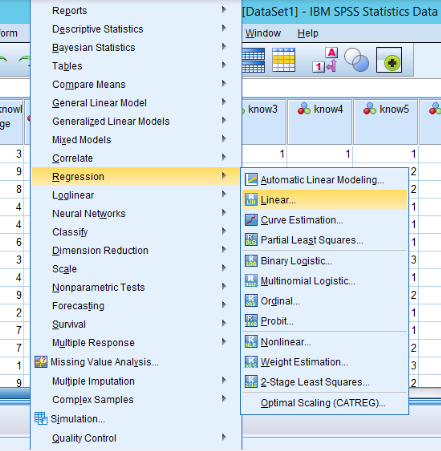
1. Select Analyze > Regression > Linear

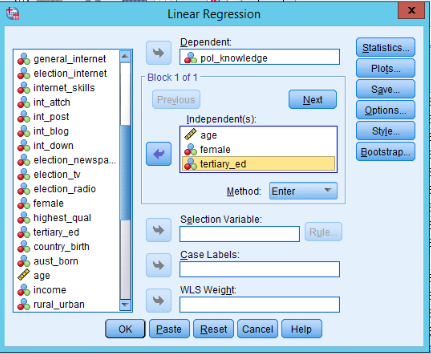
2. Select the dependent variable and put it in the top box

3. When you run HEIRARCHICAL models, you need to divide your independent variables into groups.

Select the FIRST SET of independent variables and put these in the ‘Independent(s)’ box

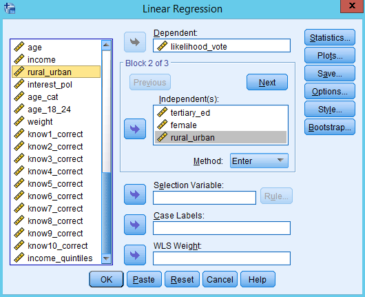
4. Press the ‘Next’ button. The independent variables box will clear.

5. Select the SECOND SET of independent variables and put these in the ‘Independent(s)’ box

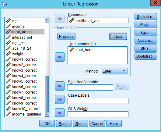
6. Press the ‘Next’ button. The independent variables box will clear.

7. Select the THIRD SET of independent variables and put these in the ‘Independent(s)’ box

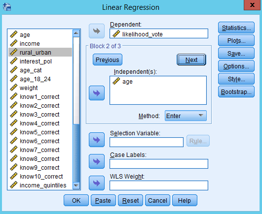
6. Press OK. The regression will run and the output screen will appear

7. How do you interpret a hierarchical linear regression?

The simplest way to think about it is that each of Model 1, Model 2, and Model 3 are completely separate FORCED ENTRY models.

The coefficients for each variable in the three models are interpreted as ‘controlling for all the other variables in the model’. The difference with the later models (like Model 3) is that there are more controls (and more variables with coefficients).

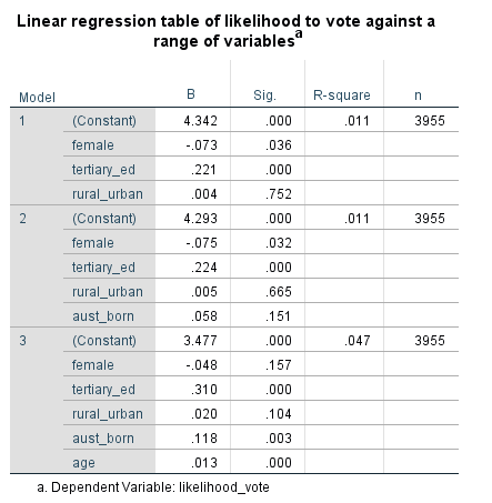
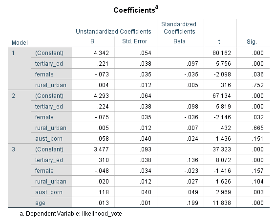
So how would we interpret this set of models?

1. Look in the ‘Sig.’ column for the p-values

2. If the p-value < 0.05 then the independent variable has a significant impact on the dependent variable

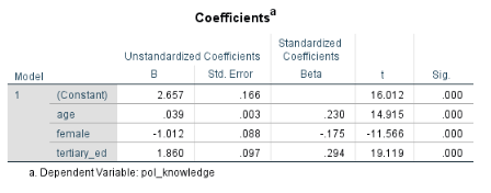
3. For the significant variables, we then read the B values (coefficients), which are the effect of a one unit increase of the independent variable on the dependent variable.

4. In this case the dependent variable is a scale from 1 to 5 with a higher number representing a lower likelihood to vote if voting was not compulsory.

5. Let’s look at the transition of one variable - female - over the three models. Female is a binary variable with 0 meaning male and 1 meaning female.

6. In models 1 and 2, female is statistically significant (Sig. column p, 0.036 and 0.032 respectively).

2. In model 3, female becomes statistically insignificant (p = 0.157). Why? Because we added the variable age. When we control for age, gender (the variable called female) is no longer statistically relevant.

3. The fact that female loses significance when we add age suggests that the variables are related. A possible interpretation is this:

‘Women are more likely to vote (if voting was not compulsory) than men, but the reason this dataset shows this is that the male sample group is skewed towards a higher age than the female group (you can see this by doing a paired t test of age by gender or by comparing the historgram of age by gender). As people get older, they are less likely to vote (if voting is not compulsory). When controlling for the age of the respondents, gender is no longer statistically relevant. So women are more likely to vote but only because they are younger (in this sample).’

(c) Stepwise regression

WARNING: YOU SHOULD PROBABLY NOT BE RUNNING A STEPWISE REGRESSION WHY? BECAUSE THEY ARE A-THEORETICAL, AND SO PRONE TO MASSIVE CONCEPTUAL FLAWS.

Let me show you through an example:

1. Select Analyze > Regression > Linear

2. Select the dependent variable and put it in the top box

3. When you run STEPWISE models, you tend to put a lot of variables into the model. You don’t generally have multiple blocks.

Select the independent variables and put these in the ‘Independent(s)’ box

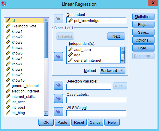
4. Under the independent variables, there is the label ‘Method’. Select ‘Backward’ from the dropdown menu.

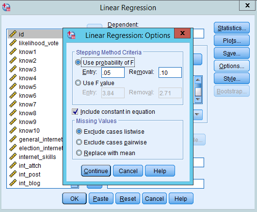
5. Click on ‘Options’.

This will reveal the options for ‘Stepping’. Because we are doing ‘Backwards selection’, you can just look at the ‘Removal’ box. Variables with Significance (p-value) greater than 0.10 will be removed from the model, one at a time. If you want you can adjust this up or down. Press ‘Continue’. Then press OK and run the model

6. How do you interpret stepwise linear regression?

First you need to wade through the huge mass of output.

The way a stepwise backwards selection regression works is that SPSS estimates a complete model with all the variables, and then if any variables have a significance of greater than 0.10, then it removes the one with the highest p-value (i.e. the least significant variable is removed). It then re-estimates the model, and repeats this process until only variables with p-values < 0.10 are left.

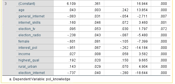
So generally we interpret a STEPWISE model by just interpreting the LAST model as a FORCED ENTRY model.

Here is the last model for our example. Notice the 3 next to the word (Constant). This is the model numbers, and this means that the method has dropped out 2 variables before getting to the final model. Dependending on how many variables you put in and their statistical relevance you could go through dozens of models.

So how would we interpret this set of models?

1. Look in the ‘Sig.’ column for the p-values

2. If the p-value < 0.05 then the independent variable has a significant impact on the dependent variable

3. Almost all the variables are significant at p < 0.05 level. But does this mean that we should SAY that these variables are a significant CAUSE of respondents’ political knowledge? What about the variables that have been excluded?

The Australian born variable was excluded in the first model because it had a p value over 0.10. But as we saw in the hierarchical model we did previously, the Australian born variable is interacting with other predictor variables. By running the hierarchical linear regression we were able to isolate that relationship, however in this stepwise regression method we are not able to to this.

THIS IS THE PROBLEM WITH STEPWISE MODELS: THEY DON’T DO THE THINKING FOR YOU, AND IF YOU GIVE IT SILLY MODELS, IT WILL STILL RUN THEM.