1.1 Multilevel modelling with the tools we already have

Now multilevel modelling is associated with a whole body of complex advanced statistics (much of which is nicely hidden from us by R and textbook explanations).

However, we can do basic multilevel modelling with the tools that we already have learnt in this course.

The main way we can do this is by including a ‘dummy’ variable for each case of the context (e.g. for each school).

1.2. Some terminology

There is a lot of confusing terminology when it comes to multilevel modelling. I will try to provide a simplified glossary for you here. Not everything will make sense now but it will be useful to refer back to later, hopefully.

Level 1: This is the smallest or micro unit of analysis. For example, if we are analysing students who are nested within schools, then students are the Level 1 cases.

Level 2: This is the next largest unit of analysis. For example, if we analysing students withing schools, schools are the Level 2 cases. This is also called a ‘context’, or ‘group’.

Level 3: We can have more levels - 3, 4, 5, etc - with each level being a larger context, within which the cases of the previous level are nested. For example, schools could be nested within districts (Level 3), which are nested within states (Level 4), which are nested within nations (Level 5).

Contexts or groups: These are the units of analysis of one of the higher levels of the models, such as the school or nation.

Fixed coefficients: These are the normal sort of coefficients we are used to using in linear and logistic regression models. They are called ‘fixed’ because there is assumed to be one value for the coefficient (which we may not know, but we are trying to estimate) which applies to all cases (e.g. persons) in the model.

Example 1: We have the cooefficient for hours of study on maths score. This will be a number (a coefficient) which says - on average - how much higher (or lower) a person scores on a maths test for each extra hour of studying then do.

Example 2: We could also have a model where we put in dummy variables for each school - Hurstville Boys, Sydney Grammar, Penrith High, etc. - and estimate the average increase (or decrease) in maths score for students who attend each school. Students at School 1 might get an average of 2.5 marks higher in the maths test, while students at School 2 might get an average of 5 marks lower.

In both example 1 and example 2, the coefficients for the variables (hours study, and for each school (a dummy variable - 1/0)) are said to be ‘fixed’ because they apply uniformly to all cases, and there is no particular assumed ‘pattern’ or distribution to the coefficients themselves.

Random coefficients: These are the main alternative to Fixed coefficients. The word ‘random’ here is a bit misleading. It probably should say ‘normally distributed coefficients’ - meaning that the coefficients themselves - at each level of the model (e.g. school) are themselves normally distributed, like a variable.

What this means is that if, for example, we had 20 schools, and we were modelling the effect of schools on maths test results, we would have a choice:

1. to model the each school as a fixed effect (i.e. dummy variable), where each school has an independent effect on math test scores. The coefficients of each school would have no particular structure or distribution. The coefficients could be clustered, or unclustered - they would not be normally distributed.
2. to model the effect of schools as a random coefficient, where the distribution of coefficients for each school has a normal distribution, and where the variance of that distribution of coefficients is estimated.

2.1 Model with homework - standard linear regression

This is a standard model of maths test score, with each student treated as an independent (not nested) case. Source: Table 2.3, page 27, (Kreft and De Leeuw, 1998)

model1 <- lm(math ~ homework, data = imm10)
summary(model1)

## 
## Call:
## lm(formula = math ~ homework, data = imm10)
## 
## Residuals:
##     Min      1Q  Median      3Q     Max 
## -28.933  -6.646   0.354   7.067  20.926 
## 
## Coefficients:
##             Estimate Std. Error t value Pr(>|t|)    
## (Intercept)   44.074      0.989    44.6   <2e-16 ***
## homework       3.572      0.388     9.2   <2e-16 ***
## ---
## Signif. codes:  0 '***' 0.001 '**' 0.01 '*' 0.05 '.' 0.1 ' ' 1
## 
## Residual standard error: 9.68 on 258 degrees of freedom
## Multiple R-squared:  0.247,  Adjusted R-squared:  0.244 
## F-statistic: 84.6 on 1 and 258 DF,  p-value: <2e-16

We can visualise this model with a simple graph

palette(rainbow(10)) 
gg <- ggplot(imm10, aes(y = math, x = homework)) +
  geom_smooth(method = lm, color = "black") +
  geom_point(size = 1.5, alpha = 0.8, colour=factor(imm10$schnum)) +
  theme(legend.position="none") 
print(gg)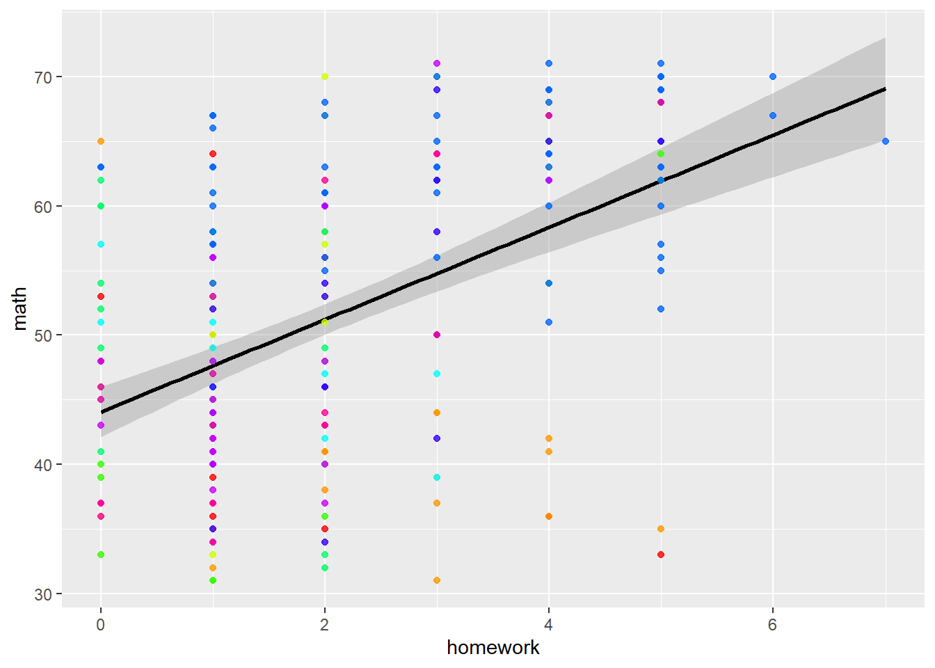

2.2 Standard linear regression - with ‘fixed coefficients’ for schools

We can now do a simple ‘fixed coefficients’ multilevel model, by running a standard linear regression model with schools as dummies

model2 <- lm(math ~ homework + as.factor(schnum), data = imm10)
summary(model2)

## 
## Call:
## lm(formula = math ~ homework + as.factor(schnum), data = imm10)
## 
## Residuals:
##     Min      1Q  Median      3Q     Max 
## -20.450  -5.055  -0.131   4.714  27.871 
## 
## Coefficients:
##                     Estimate Std. Error t value     Pr(>|t|)    
## (Intercept)           42.766      1.759   24.32      < 2e-16 ***
## homework               2.137      0.384    5.57 0.0000000660 ***
## as.factor(schnum)2    -5.638      2.485   -2.27       0.0241 *  
## as.factor(schnum)3     6.566      2.351    2.79       0.0056 ** 
## as.factor(schnum)4    -2.717      2.399   -1.13       0.2583    
## as.factor(schnum)5     5.252      2.405    2.18       0.0299 *  
## as.factor(schnum)6     1.176      2.459    0.48       0.6328    
## as.factor(schnum)7    13.007      2.075    6.27 0.0000000016 ***
## as.factor(schnum)8     2.423      2.441    0.99       0.3217    
## as.factor(schnum)9     0.718      2.426    0.30       0.7675    
## as.factor(schnum)10    1.665      2.458    0.68       0.4989    
## ---
## Signif. codes:  0 '***' 0.001 '**' 0.01 '*' 0.05 '.' 0.1 ' ' 1
## 
## Residual standard error: 8.04 on 249 degrees of freedom
## Multiple R-squared:  0.499,  Adjusted R-squared:  0.479 
## F-statistic: 24.8 on 10 and 249 DF,  p-value: <2e-16

We can visualise this model with the following code:

imm10$FEPredictions <- fitted(model2)
ml_est <- coef(summary(model2))[ , "Estimate"]
ml_se <- coef(summary(model2))[ , "Std. Error"]

palette(rainbow(10)) 
gg <- ggplot(imm10, aes(y = math, x = homework)) +
  geom_line(aes(y = FEPredictions, color=as.factor(schnum))) +
  geom_abline(slope = ml_est[2], intercept = ml_est[1], size=1) +
  geom_point(size = 1.5, alpha = 0.8, colour=factor(imm10$schnum)) +
  theme(legend.position="none") 
print(gg)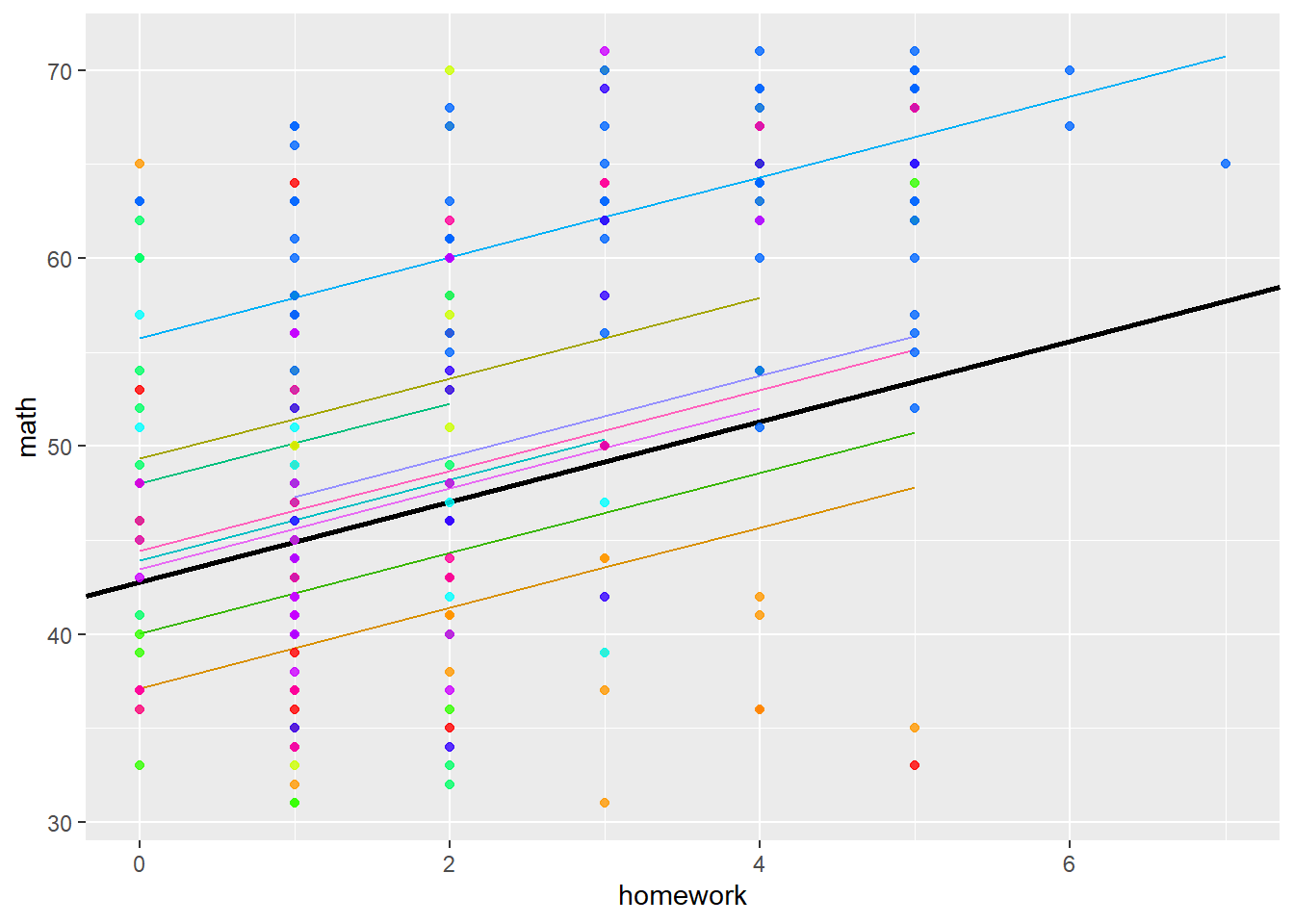

We can draw a dot-and-whisker plot

dwplot(model2,colour = "grey60") + # plots the coefficients
  geom_vline(xintercept = 0, alpha = .3) +  # puts a transparent grey line at zero
  theme_bw() + # a theme that looks nice
  scale_colour_grey() +  # makes it a bit nicer in black and white
  theme(legend.position="none") # gets rid of legend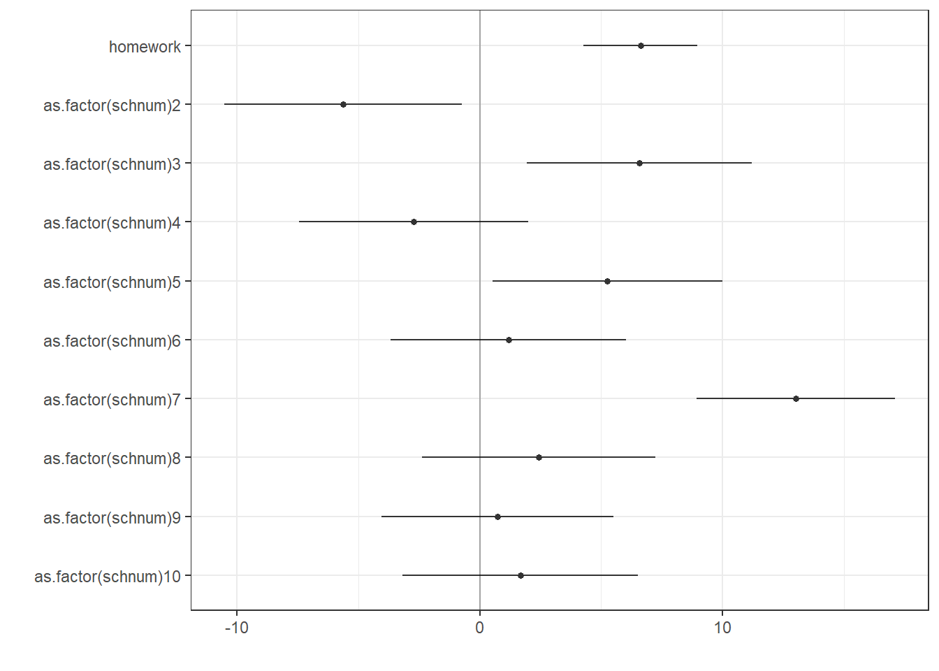

2.3 Random coefficients with lmer() function

We can also run a ‘random coefficients’ multilevel model, with the lmer() function.

This is what is called a ‘random intercept’ model, because we only allow the intercept of the schools to vary.

model3 <- lmer(math ~ homework + (1|schnum), REML=FALSE, data = imm10)
summary(model3)

## Linear mixed model fit by maximum likelihood  ['lmerMod']
## Formula: math ~ homework + (1 | schnum)
##    Data: imm10
## 
##      AIC      BIC   logLik deviance df.resid 
##     1851     1865     -921     1843      256 
## 
## Scaled residuals: 
##    Min     1Q Median     3Q    Max 
## -2.618 -0.697 -0.024  0.599  3.374 
## 
## Random effects:
##  Groups   Name        Variance Std.Dev.
##  schnum   (Intercept) 22.5     4.74    
##  Residual             64.3     8.02    
## Number of obs: 260, groups:  schnum, 10
## 
## Fixed effects:
##             Estimate Std. Error t value
## (Intercept)   44.978      1.725   26.08
## homework       2.214      0.378    5.86
## 
## Correlation of Fixed Effects:
##          (Intr)
## homework -0.387

We can visualise this model with the following code:

imm10$REPredictions <- fitted(model3)
ml_est <- coef(summary(model3))[ , "Estimate"]
ml_se <- coef(summary(model3))[ , "Std. Error"]

palette(rainbow(10)) 
gg <- ggplot(imm10, aes(y = math, x = homework)) +
  geom_line(aes(y = REPredictions, color=as.factor(schnum))) +
  geom_abline(slope = ml_est[2], intercept = ml_est[1], size=1) +
  geom_point(size = 1.5, alpha = 0.8, colour=factor(imm10$schnum)) +
  theme(legend.position="none") 
print(gg)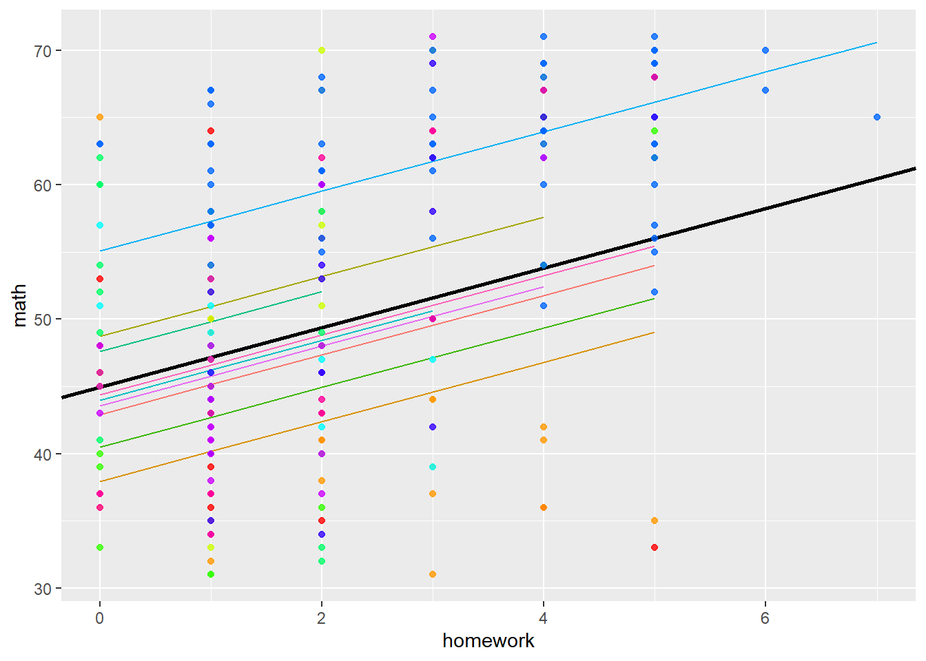

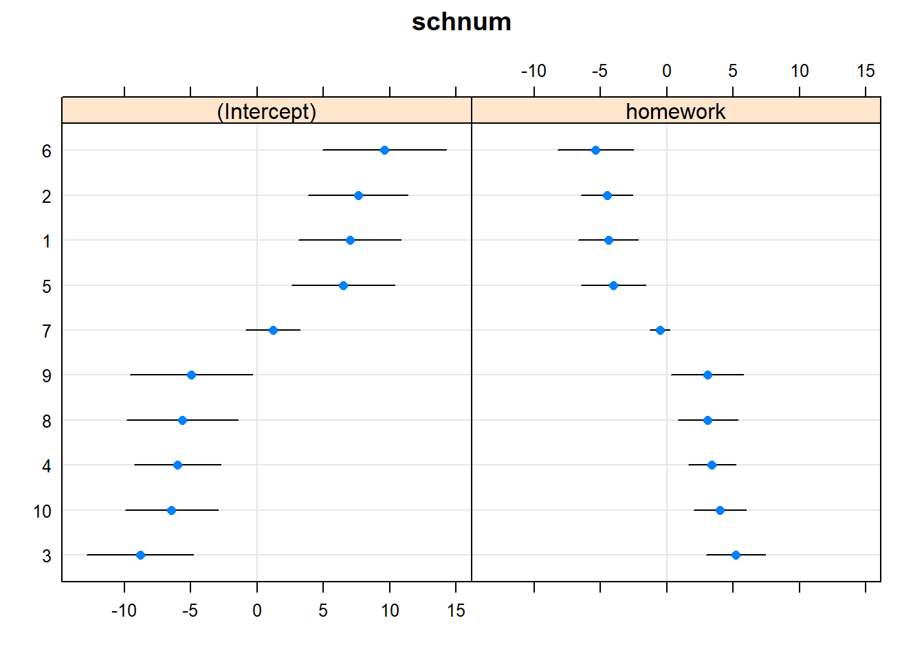
dotplot(ranef(model3, condVar=TRUE)) 

## $schnum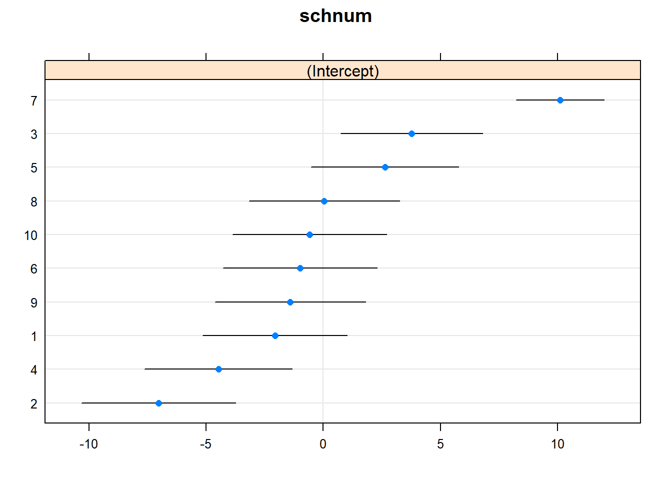

2.4 Random slope and intercept model

We can also run a ‘random slope and intercept’ multilevel model. The slopes (between maths and homework) can now vary as well.

model4 <- lmer(math ~ homework + (homework|schnum), REML=FALSE, data = imm10)
summary(model4)

## Linear mixed model fit by maximum likelihood  ['lmerMod']
## Formula: math ~ homework + (homework | schnum)
##    Data: imm10
## 
##      AIC      BIC   logLik deviance df.resid 
##     1781     1803     -885     1769      254 
## 
## Scaled residuals: 
##     Min      1Q  Median      3Q     Max 
## -2.4977 -0.5424  0.0217  0.6069  2.5711 
## 
## Random effects:
##  Groups   Name        Variance Std.Dev. Corr 
##  schnum   (Intercept) 61.8     7.86          
##           homework    20.0     4.47     -0.80
##  Residual             43.1     6.56          
## Number of obs: 260, groups:  schnum, 10
## 
## Fixed effects:
##             Estimate Std. Error t value
## (Intercept)    44.77       2.60   17.20
## homework        2.05       1.47    1.39
## 
## Correlation of Fixed Effects:
##          (Intr)
## homework -0.803

We can visualise this model with the following code:

imm10$REPredictions <- fitted(model4)
ml_est <- coef(summary(model4))[ , "Estimate"]
ml_se <- coef(summary(model4))[ , "Std. Error"]

palette(rainbow(10)) 
gg <- ggplot(imm10, aes(y = math, x = homework)) +
  geom_line(aes(y = REPredictions, color=as.factor(schnum))) +
  geom_abline(slope = ml_est[2], intercept = ml_est[1], size=1) +
  geom_point(size = 1.5, alpha = 0.8, colour=factor(imm10$schnum)) +
  theme(legend.position="none") 
print(gg)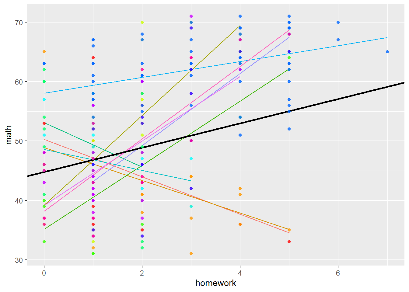

dotplot(ranef(model4, condVar=TRUE))

## $schnum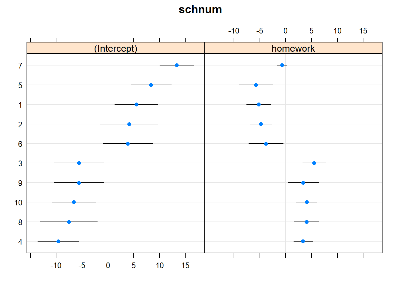

2.5 Level 1 and Level 2 Fixed Variables + Level 3 Random variable (optional)

We can now make the model more complex, by including, for example SES effects - both at the individual (ses) and school level (meanses). And we can add a third level ‘region’.

model5 <- lmer(math ~ homework + ses + meanses + (homework|schnum), REML=FALSE, data = imm10)
summary(model5)

## Linear mixed model fit by maximum likelihood  ['lmerMod']
## Formula: math ~ homework + ses + meanses + (homework | schnum)
##    Data: imm10
## 
##      AIC      BIC   logLik deviance df.resid 
##     1752     1780     -868     1736      252 
## 
## Scaled residuals: 
##     Min      1Q  Median      3Q     Max 
## -2.6575 -0.6750  0.0345  0.6360  2.6514 
## 
## Random effects:
##  Groups   Name        Variance Std.Dev. Corr 
##  schnum   (Intercept) 49.2     7.01          
##           homework    17.1     4.13     -0.99
##  Residual             41.3     6.43          
## Number of obs: 260, groups:  schnum, 10
## 
## Fixed effects:
##             Estimate Std. Error t value
## (Intercept)   48.022      2.352   20.42
## homework       1.802      1.360    1.33
## ses            2.376      0.636    3.74
## meanses        6.230      1.020    6.11
## 
## Correlation of Fixed Effects:
##          (Intr) homwrk ses   
## homework -0.973              
## ses       0.042 -0.037       
## meanses   0.066 -0.009 -0.611

dotplot(ranef(model5, condVar=TRUE))

## $schnum

References

- Chapter 19: ‘Multilevel linear models’ in Field, Miles, and Field, 2012. Discovering Statistics Using R.
- G.G. Kreft and J. De Leeuw. Introducing Multilevel Modeling, number 1 of Introducing Statistical Methods. Sage Publications, London, 1998. http://www.stat.ucla.edu/~deleeuw/janspubs/1998/books/kreft_deleeuw_B_98.pdf
- Mark Tranmer, 2010. “What is Multilevel Modelling?” https://www.youtube.com/watch?v=_lrB-ZaLQE0
- Institute for Digital Research and Education, n.d. ‘Textbook Examples Introduction to Multilevel Modeling by Kreft and de Leeuw’ https://stats.idre.ucla.edu/other/examples/imm/
0. Code to run to set up your computer.
# Update Packages
update.packages(ask = FALSE, repos='https://cran.csiro.au/', dependencies = TRUE)
# Install Packages
if(!require(dplyr)) {install.packages("dplyr", repos='https://cran.csiro.au/', dependencies=TRUE)}
if(!require(sjlabelled)) {install.packages("sjlabelled", repos='https://cran.csiro.au/', dependencies=TRUE)}
if(!require(sjmisc)) {install.packages("sjmisc", repos='https://cran.csiro.au/', dependencies=TRUE)}
if(!require(sjstats)) {install.packages("sjstats", repos='https://cran.csiro.au/', dependencies=TRUE)}
if(!require(sjPlot)) {install.packages("sjPlot", repos='https://cran.csiro.au/', dependencies=TRUE)}
if(!require(ggplot2)) {install.packages("ggplot2", repos='https://cran.csiro.au/', dependencies=TRUE)}
if(!require(ggrepel)) {install.packages("ggrepel", repos='https://cran.csiro.au/', dependencies=TRUE)}
if(!require(lme4)) {install.packages("lme4", repos='https://cran.csiro.au/', dependencies=TRUE)}
if(!require(dotwhisker)) {install.packages("dotwhisker", repos='https://cran.csiro.au/', dependencies=TRUE)}
if(!require(broom)) {install.packages("broom", repos='https://cran.csiro.au/', dependencies=TRUE)}
if(!require(lattice)) {install.packages("lattice", repos='https://cran.csiro.au/', dependencies=TRUE)}
# Load packages into memory
library(dplyr)
library(sjlabelled)
library(sjmisc)
library(sjstats)
library(sjPlot)
library(ggplot2)
library(ggrepel)
library(lme4)
library(dotwhisker)
library(broom)
library(lattice)
# Turn off scientific notation
options(digits=3, scipen=8)
# Stop View from overloading memory with a large datasets
RStudioView <- View
View <- function(x) {
if ("data.frame" %in% class(x)) { RStudioView(x[1:500,]) } else { RStudioView(x) }
}
# Datasets
# Example 1: Crime Dataset
lga <- readRDS(url("https://methods101.com/data/nsw-lga-crime-clean.RDS"))
# Example 2: AuSSA Dataset
aus2012 <- readRDS(url("https://mqsociology.github.io/learn-r/soci832/aussa2012.RDS"))
# Example 3: Australian Electoral Survey
aes_full <- readRDS(gzcon(url("https://mqsociology.github.io/learn-r/soci832/aes_full.rds")))
# Example 4: AES 2013, reduced
elect_2013 <- read.csv(url("https://methods101.com/data/elect_2013.csv"))1. Theory
Multilevel modelling is a method for dealing with the fact that cases (e.g. people) in a dataset are not really statistically independent.
As Mark Tranmer in the video in the references says “People are not raffle tickets”, meaning that we - in the real social world - we have groups, contexts, and institutions in common.
Simmel wrote that individuals lie at the intersection of many social circles. These circles might be our family, our workplace, our schools, our local government area, our nation, or many other contexts.
The power of multilevel modeling is that it can take account of the fact that people or cases situated within a larger context (a level) can systematically vary together - in a way that is simply a function of that particular context.
For example, it might turn out that if we analysed HSC results students from particular schools - even when we control for all the characteristics of the students - get a higher (or lower) University Entrance Rank simply because of the school they attend.