Week 5: Bivariate Analysis, Scales & Indicies, and Dimension Reduction |
|
Learning Objectives By the end of this class, students should be able to (1) define, (2) know when to use, (3) interpret R output for, and (4) - with the assistance of methods101.com and Google - run the R commands for the following types of statistical analysis:
|
SOCI832: Lesson 5.1: Crosstabs
0. How to I get my computer set up for today’s class?
# Install Packages
if(!require(dplyr)) {install.packages("sjlabelled", repos='https://cran.csiro.au/', dependencies=TRUE)}
if(!require(sjlabelled)) {install.packages("sjlabelled", repos='https://cran.csiro.au/', dependencies=TRUE)}
if(!require(sjmisc)) {install.packages("sjmisc", repos='https://cran.csiro.au/', dependencies=TRUE)}
if(!require(sjstats)) {install.packages("sjstats", repos='https://cran.csiro.au/', dependencies=TRUE)}
if(!require(sjPlot)) {install.packages("sjlabelled", repos='https://cran.csiro.au/', dependencies=TRUE)}
if(!require(summarytools)) {install.packages("summarytools", repos='https://cran.csiro.au/', dependencies=TRUE)}
if(!require(ggplot2)) {install.packages("ggplot2", repos='https://cran.csiro.au/', dependencies= TRUE)}
if(!require(ggthemes)) {install.packages("ggthemes", repos='https://cran.csiro.au/', dependencies= TRUE)}


# Load packages into memory
library(dplyr)
library(sjlabelled)
library(sjmisc)
library(sjstats)
library(sjPlot)
library(summarytools)
library(ggplot2)
library(ggthemes)

# Turn off scientific notation
options(digits=5, scipen=15)

# Stop View from overloading memory with a large datasets
RStudioView <- View
View <- function(x) {
  if ("data.frame" %in% class(x)) { RStudioView(x[1:500,]) } else { RStudioView(x) }
}
1. How do I make ‘crosstabs’, i.e. cross tabulate data?
In this section we look at how to cross-tabulate the levels of two variables. This is often one of the simplest ways to get a quick look at the relationship between two variables
1.1. Example 1: Political Knowledge and Likelihood of Voting
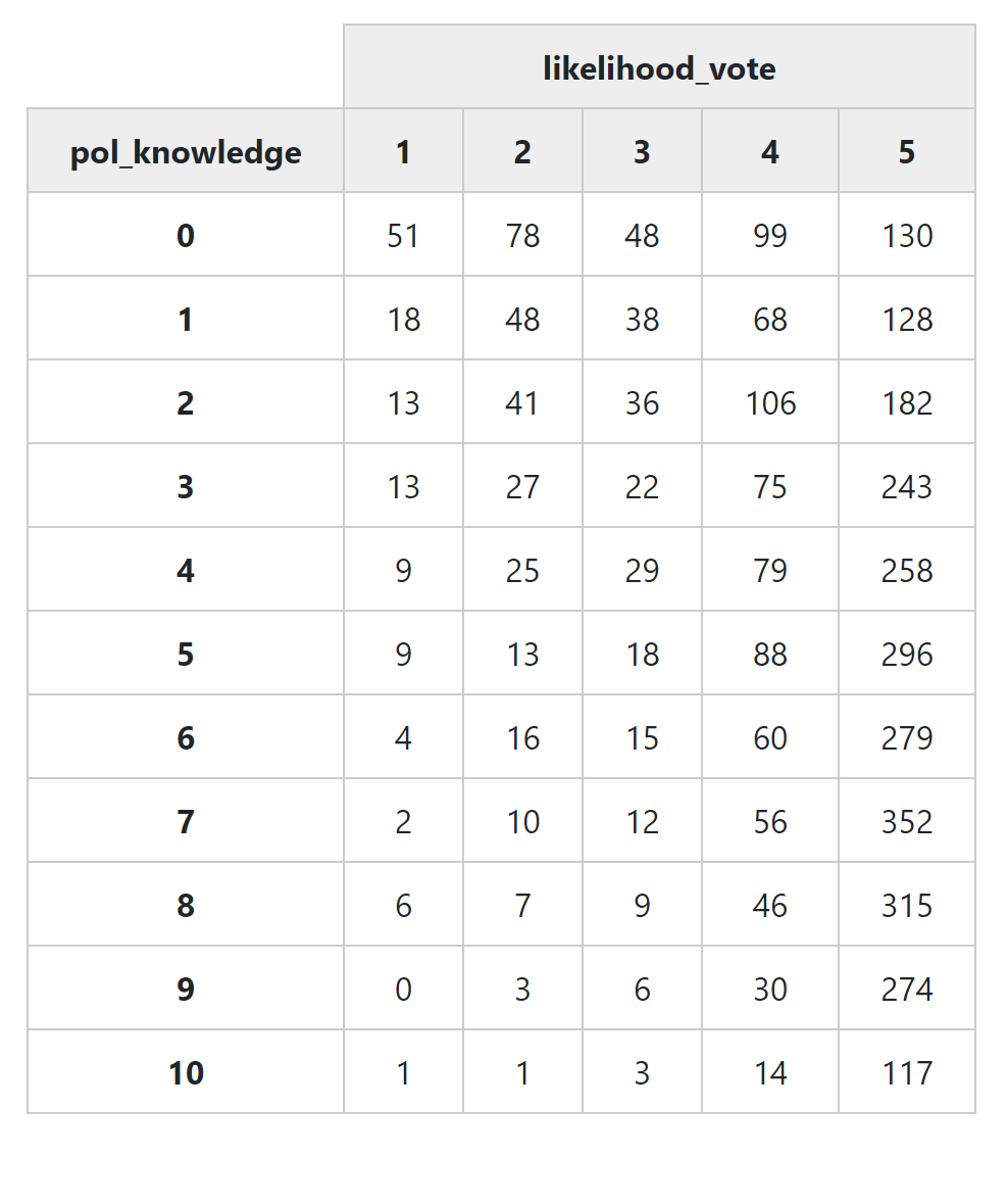
This is how the command ‘ctable()’ presents a cross tabulation with default settings:
elect_2013 <- read.csv(url("https://methods101.com/data/elect_2013.csv"))print(ctable(elect_2013$pol_knowledge,
elect_2013$likelihood_vote),
method = "browser")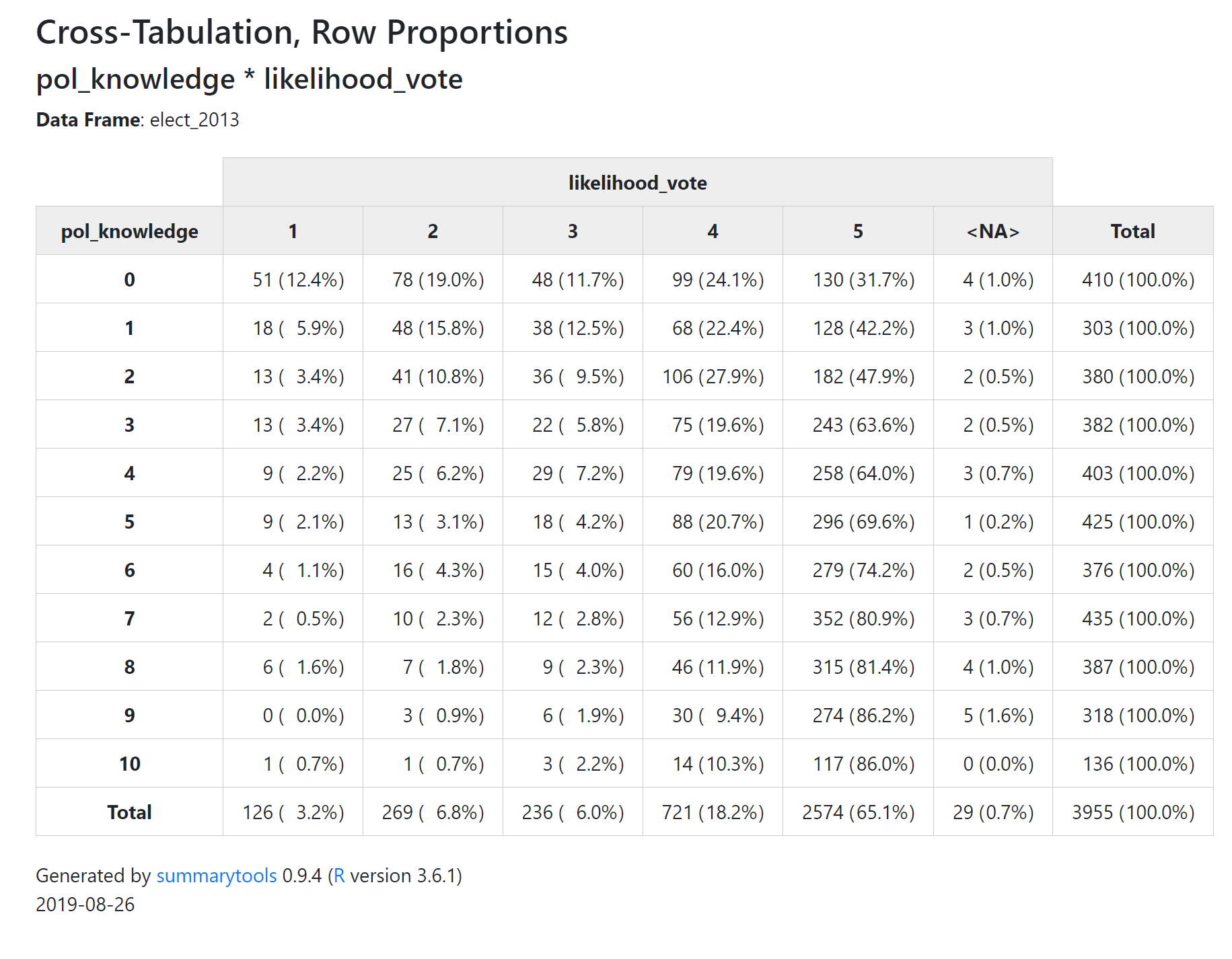
Notice that each cell in the table has two numbers the first number is the number of survey respondents who had those two values of the two variables. For exampke, there are 51 people who got zero on the political knowledge quiz, and who also said their likelihood of voting if voting was not compulsory was ‘definitely not’ (i.e. a 1 on a 5 point scale).
The second number in each cell (contained in brackets) is a percentage. In this default setting, this is the row percentage - the percentage of people with a political knowledge score of zero, who have a ‘1’ on the ‘likelihood_vote’ variable. You can see that this is 12.44%.
Often when reading cross tabulations it can be difficult to work out whether the percentages are row or column percentages. One of the easiest ways to work this out is to simply look at the ‘Total’ column, and ‘Total’ row. Almost always you will find that one of the two Totals is equal to 100% for all values of a variable. The total with the 100% is the denominator for all cells in its row or column.
So in this case, we can see that the Total column has 100% for all variables, telling you that the percentages are “percent of people with political knowledge of X, who had a likelihood of voting of Y.”
1.2. How do I get column and row percentages?
We can control the displaying of row and column percentages with the argument ‘prop’. prop takes four different settings “r” for ’row percentages is the default (so you don’t need to put this setting in).
The other options are:
- “c” for column totals (cell count/column count)
- “t” for displaying percent of all cases (cell count/total count)
- “n” for none - no percentages
So this command displays column totals
print(ctable(elect_2013$pol_knowledge,
             elect_2013$likelihood_vote,
             prop = "c"),
      method = "browser", footnote = NA)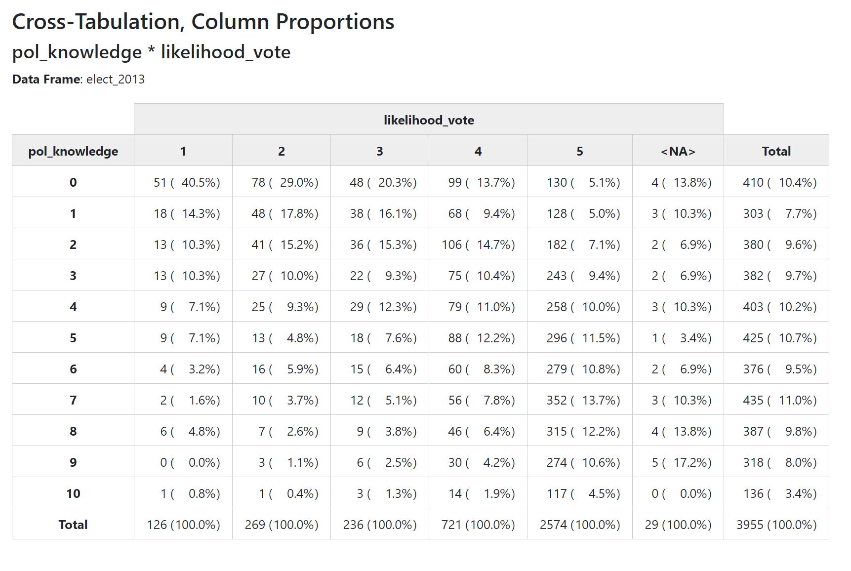
1.3 How to I get percentage of total cases in each cell?
print(ctable(elect_2013$pol_knowledge,
             elect_2013$likelihood_vote,
             prop = "t"),
      method = "browser", footnote = NA)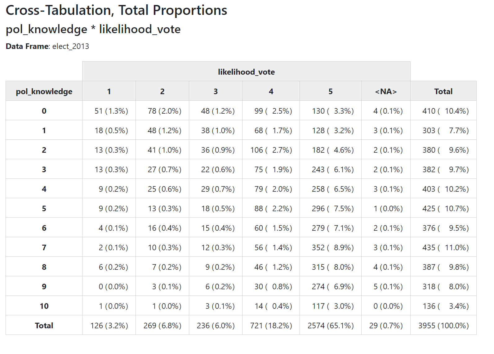
1.4 How to I get rid of percentages?
print(ctable(elect_2013$pol_knowledge,
             elect_2013$likelihood_vote,
             prop = "n"),
      method = "browser", footnote = NA)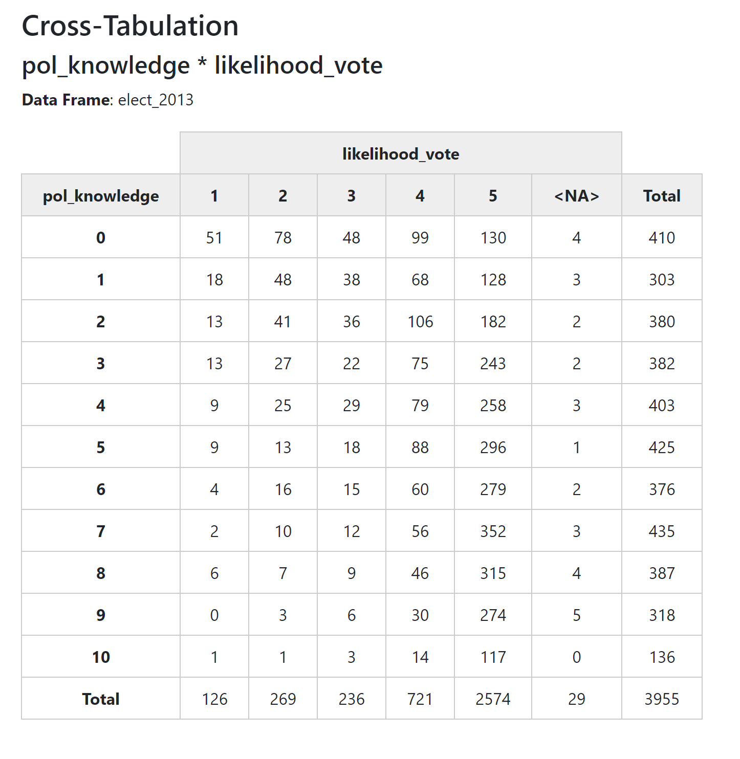
1.5 How do I make my table clean and pretty? No headings? No totals? No NAs?
As with the other summarytools functions, you can use various arguments to clean up the display of your table.
Note that for some reason we use the argument ‘useNA’ rather than ‘report.nas’ to remove NAs from our table.
print(ctable(elect_2013$pol_knowledge,
             elect_2013$likelihood_vote,
             headings = FALSE,
             totals = FALSE,
             useNA = "no",
             prop = "n"),
      method = "browser", footnote = NA)