0. Code to run to set up your computer.
# Update Packages
# update.packages(ask = FALSE, repos='https://cran.csiro.au/', dependencies = TRUE)

# Install Packages
if(!require(dplyr)) {install.packages("sjlabelled", repos='https://cran.csiro.au/', dependencies=TRUE)}
if(!require(sjlabelled)) {install.packages("sjlabelled", repos='https://cran.csiro.au/', dependencies=TRUE)}
if(!require(sjmisc)) {install.packages("sjmisc", repos='https://cran.csiro.au/', dependencies=TRUE)}
if(!require(sjstats)) {install.packages("sjstats", repos='https://cran.csiro.au/', dependencies=TRUE)}
if(!require(sjPlot)) {install.packages("sjlabelled", repos='https://cran.csiro.au/', dependencies=TRUE)}
if(!require(summarytools)) {install.packages("summarytools", repos='https://cran.csiro.au/', dependencies=TRUE)}
if(!require(ggplot2)) {install.packages("ggplot2", repos='https://cran.csiro.au/', dependencies= TRUE)}
if(!require(ggthemes)) {install.packages("ggthemes", repos='https://cran.csiro.au/', dependencies= TRUE)}
if (!require(GPArotation)) install.packages("GPArotation", repos='https://cran.csiro.au/', dependencies = TRUE)
if (!require(psych)) install.packages("psych", repos='https://cran.csiro.au/', dependencies = TRUE)
if (!require(ggrepel)) install.packages("ggrepel", repos='https://cran.csiro.au/', dependencies = TRUE)


# Load packages into memory
library(dplyr)
library(sjlabelled)
library(sjmisc)
library(sjstats)
library(sjPlot)
library(summarytools)
library(ggplot2)
library(ggthemes)
library(GPArotation)
library(psych)
library(ggrepel)

# Turn off scientific notation
options(digits=5, scipen=15)

# Stop View from overloading memory with a large datasets
RStudioView <- View
View <- function(x) {
  if ("data.frame" %in% class(x)) { RStudioView(x[1:500,]) } else { RStudioView(x) }
}

# Datasets
# Example 1: Crime Dataset
lga <- readRDS(url("https://methods101.com/data/nsw-lga-crime-clean.RDS"))
# extract just the crimes from crime dataset
first <- which( colnames(lga)=="astdomviol" )
last <- which(colnames(lga)=="transport")
crimes <- lga[, first:last ]

# Example 2: AuSSA Dataset
aus2012 <- readRDS(url("https://mqsociology.github.io/learn-r/soci832/aussa2012.RDS"))

# Example 3: Australian Electoral Survey
aes_full <- readRDS(gzcon(url("https://mqsociology.github.io/learn-r/soci832/aes_full.rds")))
# Codebook
browseURL("https://mqsociology.github.io/learn-r/soci832/aes_full_codebook.html")
1. Table of Factor Loadings
# We could just do this all with one command
sjt.fa(crimes, nmbr.fctr = 3, rotation = c("promax"), method="minres")
## Warning in cor.smooth(R): Matrix was not positive definite, smoothing was
## done

## Warning in cor.smooth(R): Matrix was not positive definite, smoothing was
## done

## Warning in cor.smooth(R): Matrix was not positive definite, smoothing was
## done
## Warning in fac(r = r, nfactors = nfactors, n.obs = n.obs, rotate =
## rotate, : A loading greater than abs(1) was detected. Examine the loadings
## carefully.
## Warning in cor.smooth(r): Matrix was not positive definite, smoothing was
## done
## Warning in fa.stats(r = r, f = f, phi = phi, n.obs = n.obs, np.obs
## = np.obs, : The estimated weights for the factor scores are probably
## incorrect. Try a different factor extraction method.
Factor Analysis
|
|
Factor 1
|
Factor 2
|
Factor 3
|
|
Assault - domestic violence
|
0.91
|
0.03
|
-0.06
|
|
Assault - non-domestic violence
|
0.58
|
0.38
|
0.19
|
|
Sexual Offences
|
0.56
|
0.33
|
-0.12
|
|
Robbery
|
0.54
|
0.08
|
0.48
|
|
Break and entering dwelling
|
1.01
|
-0.19
|
0.07
|
|
Break and entering non-dwelling
|
0.85
|
-0.03
|
-0.08
|
|
Motor vehicle theft
|
0.95
|
-0.28
|
0.16
|
|
Steal from motor vehicle
|
0.87
|
-0.29
|
0.33
|
|
Steal from retail store
|
0.19
|
0.07
|
0.74
|
|
Steal from dwelling
|
0.78
|
0.13
|
-0.01
|
|
Steal from person
|
-0.34
|
0.55
|
0.76
|
|
Fraud
|
-0.14
|
0.03
|
0.90
|
|
Malicious damage to property
|
0.96
|
-0.00
|
0.01
|
|
Harassment and threatening
|
0.86
|
0.09
|
-0.15
|
|
Receiving stolen goods
|
0.29
|
0.16
|
0.70
|
|
Other theft
|
0.11
|
0.58
|
0.44
|
|
Arson
|
0.91
|
-0.11
|
-0.03
|
|
Possession use of cannabis
|
0.09
|
0.61
|
0.11
|
|
Prohibited weapons offences
|
0.63
|
0.20
|
-0.20
|
|
Trespass
|
0.69
|
0.26
|
-0.18
|
|
Offensive conduct
|
0.07
|
0.83
|
-0.03
|
|
Offensive language
|
0.49
|
0.49
|
-0.21
|
|
Liquor Offences
|
-0.33
|
0.92
|
0.16
|
|
Breach AVO
|
0.89
|
0.03
|
-0.18
|
|
Breach bail condition
|
0.64
|
-0.03
|
0.30
|
|
Resist or hinder officer
|
0.43
|
0.56
|
-0.02
|
|
Transport regulatory offences
|
-0.17
|
-0.12
|
0.63
|
|
Cronbach’s α
|
0.94
|
0.82
|
0.37
|
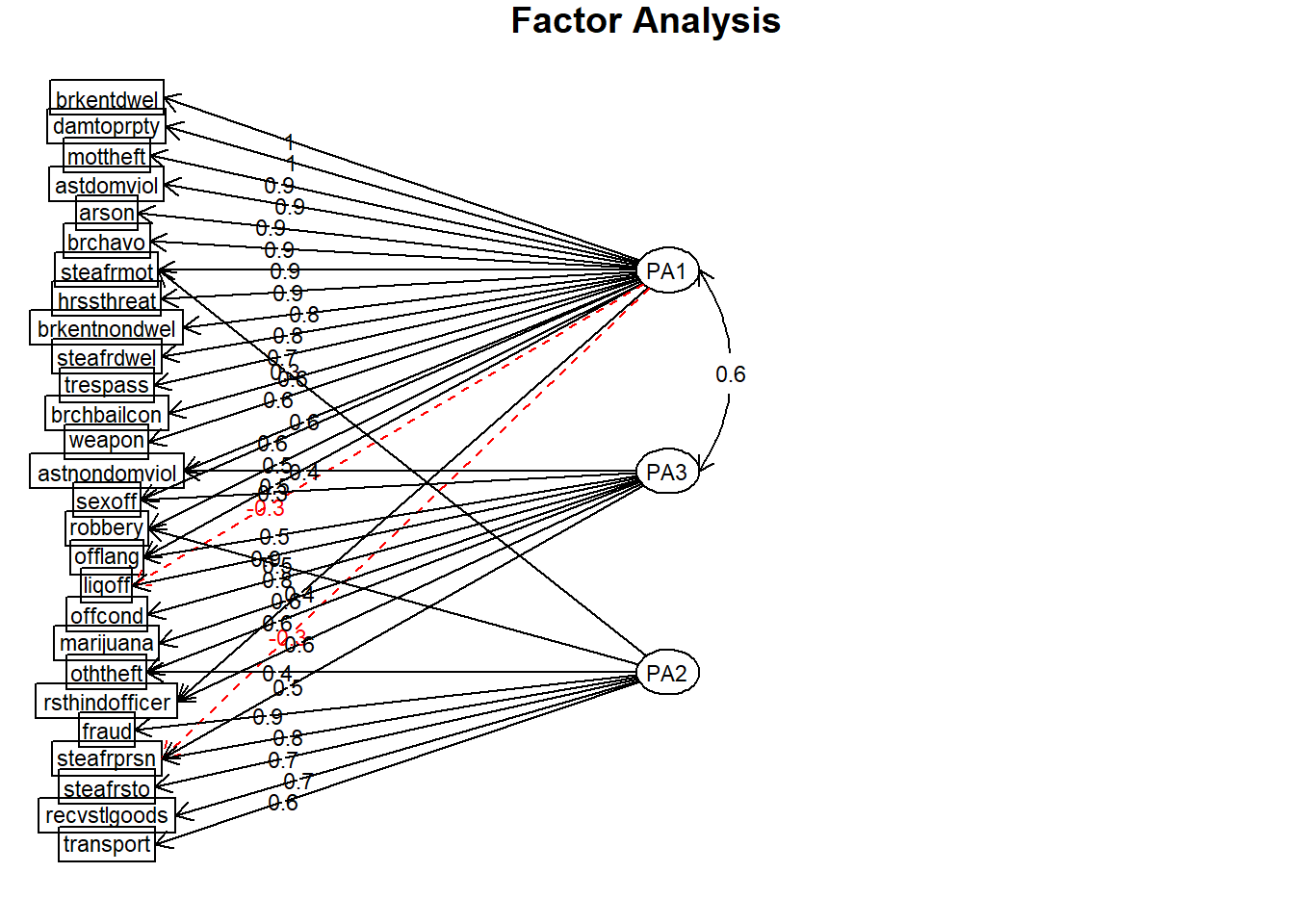
2. Visualising Factors
# (Step 4) Visualise the factors
results.1 <- psych::fa(r = crimes, nfactors = 3, rotate = "promax", fm="pa")
## Warning in cor.smooth(R): Matrix was not positive definite, smoothing was
## done
## Warning in fac(r = r, nfactors = nfactors, n.obs = n.obs, rotate =
## rotate, : A loading greater than abs(1) was detected. Examine the loadings
## carefully.
## Warning in cor.smooth(r): Matrix was not positive definite, smoothing was
## done
## Warning in fa.stats(r = r, f = f, phi = phi, n.obs = n.obs, np.obs
## = np.obs, : The estimated weights for the factor scores are probably
## incorrect. Try a different factor extraction method.
psych::fa.diagram(results.1,
    sort=TRUE,
    cut=.3,
    simple=TRUE,
    digits=1)
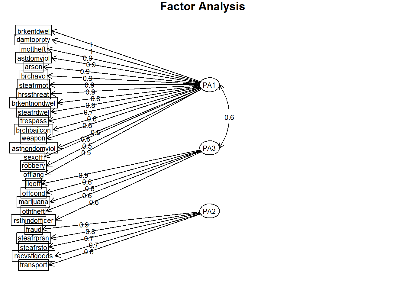
# (Step 4) Visualise the factors
psych::fa.diagram(results.1,
    sort=TRUE,
    cut=.3,
    simple=FALSE,
    digits=1)