SOCI2000 Workshop 6: Logistic Regression

Reading

‘Chapter 19: Logistic Regression’ in Andy Field, 2017. Discovering Statistics Using IBM SPSS Statistics. Sage.

Summary

We generally use logistic regressions when we have

  1. a dependent variable that is binary (i.e. it has only two values, 0 and 1), and
  2. we want to test the impact of (and/or control for) multiple independent variables.

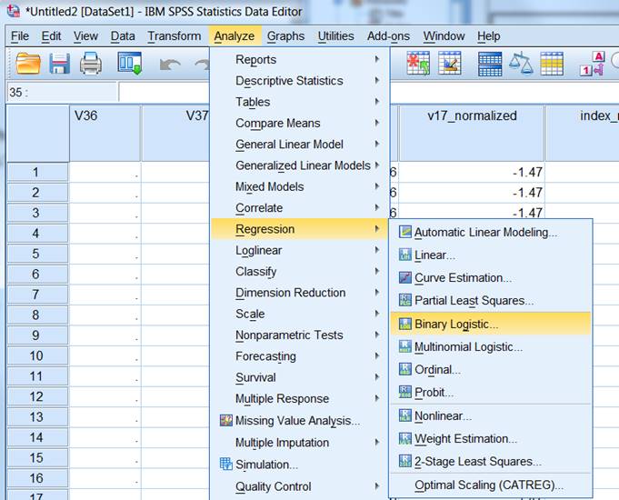
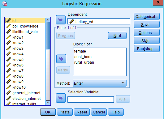
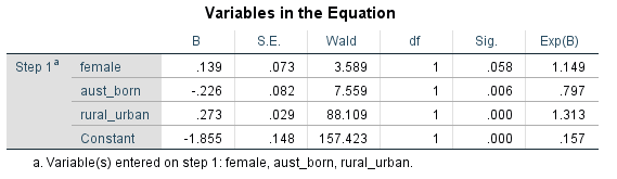
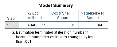
The process of running a regression in SPSS is basically the same as for linear regressions, with options for forced entry, hierarchical, and stepwise methods.

When you read your results from a regression, you read the same two columns as in a linear regression (B and sig.).

Significance (sig.) is read the same as for a linear regression.

Because of the binary nature of the dependent variable in a logistic regression, the B is not so straightforward to interpret.

B is basically a number which represents the impact of the independent variable on the probably of the dependent variable being 1.

For this course, we are only going to interpret the significance, and direction (positive or negative) of B. We won’t interpret the magnitude. So for significant (< 0.05) B coefficients we say that independent variables with positive B (greater than 0) increase the likelihood of the dependent variable being 1 (and the reverse for negative B values).

We can also view the various different R-square values for the model, which is approximately the same meaning as that for a linear regression.

Running a logistic regression

I’m just going to illustrate logistic regressions with FORCED ENTRY, because the procedure for hierarchical and stepwise methods is the same as that for linear regressions.

  1. Select Analyze > Regression > Binary Logistic…

  1. Select the dependent variable and put it in the top box

  2. Select the independent variables and put these in the ‘Independent(s)’ box.

  1. Press OK. The regression will run and the output screen will appear

  2. You can then interpret the coefficients of the regression.

  1. Look in the ‘Sig.’ column for the p-values

  2. If the p-value < 0.05 then the independent variable has a significant impact on the dependent variable

  3. For the significant variables, we then read the B values (coefficients), which are the effect of a one unit increase of the independent variable on the dependent variable.

  4. The problem with Logistic Regressions is that the independent variables DO NOT HAVE A LINEAR effect on the dependent variable. This makes the B values difficult to interpret. For this course we are not going to interpret the meaning of B values, except to ask (1) are they statistically significant; and (2) are they positive or negative, i.e. does the independent variable increase or decrease the likelihood of the dependent variable being 1 (rather than 0)

  5. In this regression we can see that female (gender) is not statistically significant (p = 0.058).

  6. Aust_born is statistically significacnt. If a person is born in Australia, they are less likely to have a tertiary education (B = -0.226).

  7. Rural_urban is statistically significant. The more urban the area the person lives in, the more likely they have a tertiary education (B = 0.273).

  1. You can find an R-square value for the regression model, in the SPSS output:

You can choose to interpret either the Cox & Snell R Square, or the Nagelkerke R Square. These basically say that between 3% and 4% of the explained variance in tertiary education for respondents is explained by our three variables (gender, australian born, and rural-urban).