1. Run the standard set up code

# Install Packages
if(!require(dplyr)) {install.packages("sjlabelled", repos='https://cran.csiro.au/', dependencies=TRUE)}
if(!require(sjlabelled)) {install.packages("sjlabelled", repos='https://cran.csiro.au/', dependencies=TRUE)}
if(!require(sjmisc)) {install.packages("sjmisc", repos='https://cran.csiro.au/', dependencies=TRUE)}
if(!require(sjPlot)) {install.packages("sjlabelled", repos='https://cran.csiro.au/', dependencies=TRUE)}
if(!require(summarytools)) {install.packages("summarytools", repos='https://cran.csiro.au/', dependencies=TRUE)}

# Load packages into memory
library(dplyr)
library(sjlabelled)
library(sjmisc)
library(sjPlot)
library(summarytools)

# Turn off scientific notation
options(digits=5, scipen=15) 

# Stop View from overloading memory with a large datasets
RStudioView <- View
View <- function(x) {
  if ("data.frame" %in% class(x)) { RStudioView(x[1:500,]) } else { RStudioView(x) }
}

2. Import using sjlabelled::read_spss or read_stata

I tend to call my datasets ds because it is short and easy to remember. ds stands for dataset.

ds <- sjlabelled::read_spss("C:\your folder\your_file.sav") 

# OR 

ds <- sjlabelled::read_stata("C:\your folder\your_file.sav") 

3. Convert to a tibble data frame object

We do this to make the data more compact and so it uses up less memory on your computer.

ds <- as_tibble(ds)

4. Create an r_codebook.html file

You want to create a codebook from your current data frame in R.

You can do this by running the following code.

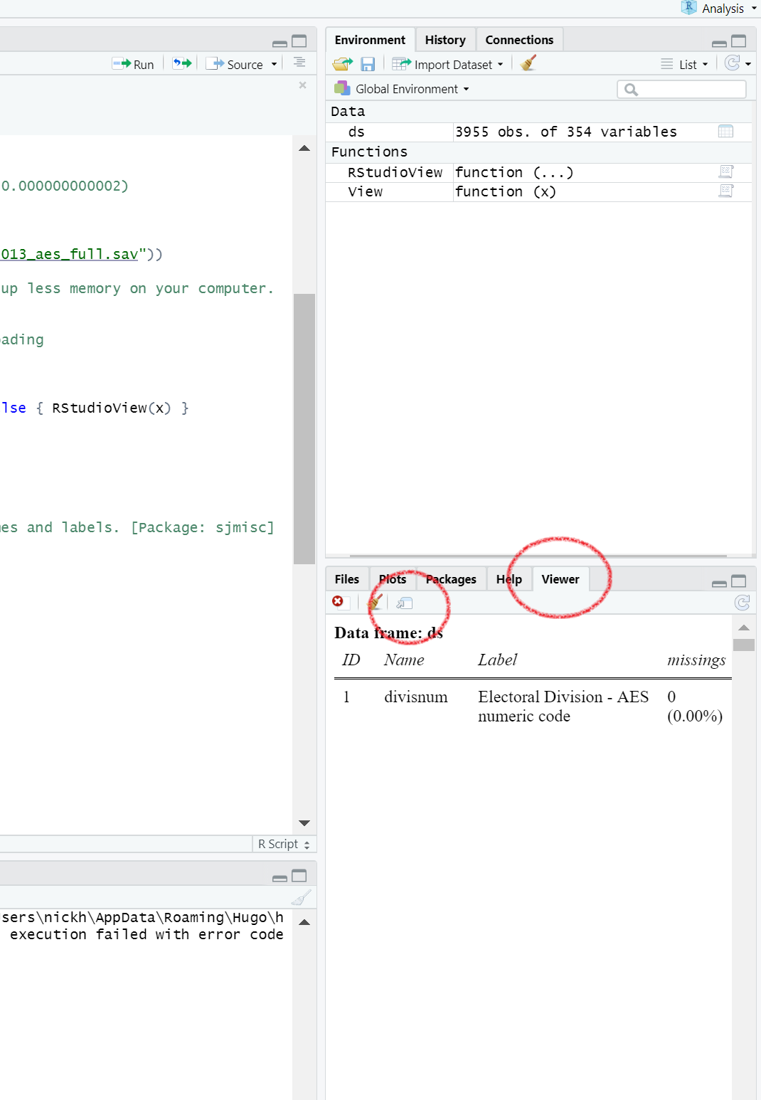
view_df(ds, show.frq = TRUE, show.na = TRUE, max.len = 300)

In the “Viewer” tab (bottom right corner of standard RStudio layout), the codebook will appear.

Click on the button with an arrow and browser window (circled in red in Figure below).

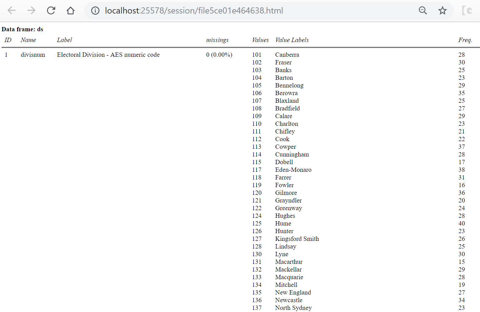
In your brower, the codebook will now open and it should look like the figure below.

In this you can see:

• Variable names
• Variable label
• Missing values
• Variable values
• Variable value labels
• Frequency of each variable value